T05: Scientific and aerospace-related computing

5 exercises, each with a complete solution. 1 figure. 1 code listing.

On this page

A. Prerequisites and observable goals
B. The central question: what exactly does this simulation claim to represent?
C. Units and nondimensionalization reduce hidden mistakes
D. Derive conservation laws before testing them
E. Velocity Verlet uses acceleration at both ends
F. Interpret the measured validation rather than a pretty curve
G. Independent practice
H. Complete solutions: T05
I. Retention and readiness

A. Prerequisites and observable goals#

Before

Calculus I–III motion and vector fields; A05 numerical error; A06 ODE integration; A01 vectors; C14 reproducibility.

After

Construct a nondimensional motion model, derive conserved quantities, validate a numerical orbit against an analytic solution, and distinguish model error from discretization and roundoff error.

Level: Advanced-entry track. A bounded idealized orbit, not mission design, flight software, or a validated aerospace tool.

B. The central question: what exactly does this simulation claim to represent?#

A scientific simulation begins with a model, its assumptions, inputs, units, numerical method, and validation target. A visually plausible trajectory is not enough. A game may deliberately sacrifice physical fidelity for responsiveness; a scientific calculation must state which physical quantities and accuracy requirements it aims to preserve. Neither purpose is inherently wrong, but their evidence standards differ.

Consider a point particle moving under a fixed central inverse-square attraction in a plane. Let position be $r=(x,y)$ , velocity $v$ , and parameter $\mu>0$ . The model is

\dot r=v,\qquad \dot v=-\mu\frac{r}{\|r\|^3},\qquad \|r\|>0.

It ignores extended bodies, collisions, atmospheric drag, propulsion, relativistic effects, and perturbations from other bodies. The origin is singular. A numerical step approaching it needs careful handling; the small circular example intentionally stays far away. We do not insert real planetary constants or claim ephemeris accuracy.

C. Units and nondimensionalization reduce hidden mistakes#

If position has units of length and time has units of time, then $\mu$ has units length $^3$ /time $^2$ , so acceleration has length/time $^2$ . Choose a reference length $R$ and time scale $T=\sqrt{R^3/\mu}$ . Writing $r=R\tilde r$ and $t=T\tilde t$ gives

\frac{\dd^2\tilde r}{\dd\tilde t^2}=-\frac{\tilde r}{\|\tilde r\|^3}.

The nondimensional model has parameter one. This does not change the physics of the specified idealization; it changes units and often improves numerical scale. Record the conversion back to physical quantities rather than mixing nondimensional coordinates with seconds or meters later.

For $\mu=1$ , initial position $(1,0)$ and velocity $(0,1)$ have exact circular solution $r(t)=(\cos t,\sin t)$ , $v(t)=(-\sin t,\cos t)$ and period $2\pi$ . Differentiate twice to verify the acceleration is $-r$ , and note that radius remains one. This analytic solution supplies a stronger validation target than a plotted loop that merely appears closed.

D. Derive conservation laws before testing them#

Specific mechanical energy is

E=\frac12\|v\|^2-\frac{\mu}{\|r\|}.

Since $\frac{\dd}{\dd t}(1/\|r\|)=-(r\cdot v)/\|r\|^3$ , differentiating energy gives

\dot E=v\cdot\left(-\mu\frac r{\|r\|^3}\right)+\mu\frac{r\cdot v}{\|r\|^3}=0.

The planar specific angular momentum is $L=xv_y-yv_x$ . Its derivative is $x a_y-y a_x$ , because the two velocity-product terms cancel. Central acceleration is parallel to $r$ , so this cross product is zero. For the unit circular initial state, $E=-1/2$ and $L=1$ .

A conserved quantity is a diagnostic, not a complete solution oracle. A method could maintain nearly constant energy while accumulating phase error. Therefore check position error against the known circle, energy variation, angular momentum variation, and convergence under step refinement. Each catches a different failure mode.

E. Velocity Verlet uses acceleration at both ends#

For acceleration depending on position, velocity Verlet advances

\begin{align*} r_{k+1}&=r_k+h v_k+\tfrac12h^2a(r_k),\\ v_{k+1}&=v_k+\tfrac12h\left[a(r_k)+a(r_{k+1})\right]. \end{align*}

The position update uses a second-order local Taylor idea. The velocity update averages endpoint accelerations. For smooth conservative mechanical systems with fixed steps, this method has useful geometric properties and second-order global accuracy under the usual regularity conditions. It does not exactly conserve the original energy for every finite step or make singular trajectories safe.

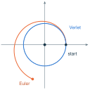
Compare it with forward Euler on an oscillator, which can systematically increase energy. A higher-order method can reduce error, but method selection also considers long-time qualitative behavior, stability, cost, and event handling. Adaptive step sizes and close encounters require additional analysis rather than simply changing $h$ whenever a plotted curve looks bad.

The companion records every state together with energy and angular momentum, rejects the singular initial origin, and uses synthetic nondimensional inputs. It is a small reference implementation for reasoning and validation, not a general orbital propagator.

The same orbit, two integrators. A body starts on the dashed unit circle at the speed that should keep it there, and both methods take 100 steps over one period. Explicit Euler gains energy at every step and spirals out to radius

1.72

. Velocity Verlet returns to within

0.008

of the start, and its energy never drifts by more than

2\times10^{-6}

F. Interpret the measured validation rather than a pretty curve#

The reference experiment used $h=2\pi/1000$ and 1000 steps, one nominal circular period. It recorded final position approximately $(0.9999999966,-0.00008268216)$ , position error $8.2682\times10^{-5}$ , maximum absolute energy deviation $1.9481\times10^{-10}$ , and maximum absolute angular-momentum deviation $1.1102\times10^{-15}$ in this environment. Tiny energy variation coexists with a larger phase-related position error, illustrating why one invariant is not enough.

Separate three errors. Modeling error comes from omitted or inaccurate physical assumptions. Discretization error comes from replacing continuous evolution with finite steps. Roundoff error comes from bounded arithmetic. Step refinement can diagnose discretization behavior but cannot fix a wrong force law or units. Agreement between two implementations of the same wrong equation is not physical validation.

For reproducibility, preserve source revision, units, parameters, initial conditions, step policy, final time, tolerances, environment, and raw diagnostics. A scientific report should explain whether comparisons use analytic truth, a higher-accuracy numerical reference, or observational data, because those are different evidence sources. Safety-critical use requires domain-specific verification, validation, and organizational processes far beyond this exercise.

G. Independent practice#

F foundation C standard course work T transfer S optional stretch L runnable lab or project. Attempt the complete set before opening its solutions.

T05.01CSolution

Verify directly that $r(t)=(\cos t,\sin t)$ satisfies the nondimensional central-force equation for all real $t$ . Compute its energy and angular momentum.

T05.02CSolution

Starting from $(r,v)=((1,0),(0,1))$ with $\mu=1$ , write the velocity-Verlet position after one step of size $h$ . Then express the next acceleration and velocity update without replacing them by Euler’s update.

T05.03TSolution

A simulation has energy error below $10^{-10}$ but misses the expected final position by $10^{-3}$ . Is that logically inconsistent? Explain what additional diagnostic is needed and identify one mistake that reducing the time step cannot repair.

T05.04CSolution

A method is in a regime with global error approximately $Ch^2$ . If an error is $8\times10^{-4}$ at step $h$ , predict the error at $h/2$ and explain why observing that ratio on one pair of runs is evidence, not a proof of the order for all problems.

T05.05LabSolution

Implement starters/orbit_lab.py: central acceleration, energy and angular momentum diagnostics, and velocity-Verlet integration. Validate the unit circular case over a nominal period, compare two step sizes, and report all three error measures. Keep the model nondimensional and reject the singular origin.

Optional small hints

For T05.01, radius is exactly one. For T05.02, the new acceleration must be evaluated at the new position. For T05.03, conservation and phase accuracy are different properties.

H. Complete solutions: T05#

Compare the first step where your work differs. A corrected answer is not yet an independent success.

T05.01Show solution

Substitute into the original differential equation

$r''=(-\cos t,-\sin t)=-r$ and $\|r\|=1$ , so $r''=-r/\|r\|^3$ . Velocity is $(-\sin t,\cos t)$ with squared speed one. Energy is $1/2-1=-1/2$ . Angular momentum is $\cos^2t+\sin^2t=1$ . The radius never vanishes, so the equation’s domain condition holds. This verifies the full trajectory, not merely its initial state.

Back to T05.01

T05.02Show solution

Use both endpoint accelerations

Initial acceleration is $(-1,0)$ . Thus $r_1=(1-h^2/2,h)$ . Let $\rho=\sqrt{(1-h^2/2)^2+h^2}$ . Then $a_1=(-(1-h^2/2)/\rho^3,-h/\rho^3)$ and

v_1=(0,1)+\frac h2\left[(-1,0)+a_1\right].

Using only the initial acceleration for velocity would give a different method. The expression preserves the distinction between a position update and a velocity update, and the denominator is nonzero for real $h$ because the two position components cannot both vanish.

Back to T05.02

T05.03Show solution

A conserved scalar does not locate the state uniquely

There is no contradiction. Many positions and velocities can share the same energy; even a nearly circular trajectory can be shifted in phase. Compare position and velocity against an analytic or independently justified reference at the same times, and inspect phase or period error. A wrong unit conversion, initial condition, or force model cannot be repaired merely by smaller steps: the method may converge accurately to the wrong modeled problem.

Back to T05.03

T05.04Show solution

A second-order prediction has a restricted meaning

Halving $h$ predicts one quarter the error, $2\times10^{-4}$ , if the leading $Ch^2$ term dominates and other assumptions remain comparable. A single ratio can be affected by cancellation, roundoff, a special initial condition, or a reference error. Test several refinements and verify regularity, stability, and a common final time. Theoretical order is a mathematical statement under hypotheses; a convergence experiment is evidence that the implementation behaves accordingly in the tested regime.

Back to T05.04

T05.05Show solution

Complete validated idealized orbit

The reference computes new acceleration only after obtaining the new position, then averages old and new accelerations for velocity. Diagnostics are stored from the initial state onward. The tests compare selected circular cases and refinement behavior; this does not validate omitted physical forces or arbitrary close approaches to the singularity.

code/solutions/orbit_lab.pyPython

"""T05.05: nondimensional two-body orbit with velocity Verlet."""
import math

def acceleration(position, mu=1.0):
    x, y = position
    r = math.hypot(x, y)
    if not math.isfinite(r) or r == 0 or not math.isfinite(mu) or mu <= 0:
        raise ValueError("finite nonzero radius and positive mu required")
    return (-mu * x / r**3, -mu * y / r**3)

def diagnostics(position, velocity, mu=1.0):
    x, y = position
    vx, vy = velocity
    r = math.hypot(x, y)
    if r == 0: raise ValueError("singular origin")
    return (0.5 * (vx*vx + vy*vy) - mu / r, x*vy - y*vx)

def orbit(dt=0.01, steps=1000, mu=1.0, position=(1., 0.), velocity=(0., 1.)):
    if type(steps) is not int or steps < 1 or not math.isfinite(dt) or dt <= 0:
        raise ValueError("positive finite step and integer step count required")
    if any(not math.isfinite(x) for x in (*position, *velocity)):
        raise ValueError("finite initial state required")
    p, v = tuple(position), tuple(velocity)
    out = [(0., p, v, *diagnostics(p, v, mu))]
    for i in range(steps):
        a = acceleration(p, mu)
        next_p = tuple(p[j] + dt*v[j] + 0.5*dt*dt*a[j] for j in range(2))
        next_a = acceleration(next_p, mu)
        v = tuple(v[j] + 0.5*dt*(a[j] + next_a[j]) for j in range(2))
        p = next_p
        out.append(((i + 1)*dt, p, v, *diagnostics(p, v, mu)))
    return out

if __name__ == "__main__":
    data = orbit(dt=2*math.pi/1000, steps=1000)
    print("one nominal circular period:", data[-1])

Back to T05.05

I. Retention and readiness#

Retrieve vector derivatives, units, numerical stability, and the distinction between invariants and full correctness. Readiness requires reproducing an analytic case and defending an error budget. Continue with deeper ODEs, numerical analysis, mechanics, uncertainty quantification, and domain-specific scientific validation before using a simulation for consequential aerospace decisions.