C07: Algorithm design, correctness, and complexity

A. Prerequisites and observable goals#

Level: Degree core.

B. The central question: why does this method solve this problem?#

An algorithm is a finite, precisely described procedure under a model of computation. An implementation selects a language, representation, and operational details. Correctness asks whether the procedure terminates with the specified result on every valid input. Complexity asks how resources grow with input size under a stated cost model. Benchmarking asks what a particular implementation does on a particular environment and workload. None of these questions substitutes for the other two.

For eventually nonnegative functions, $f(n)=O(g(n))$ means there exist constants $c,n_0$ such that $f(n)\le c g(n)$ for all $n\ge n_0$. $\Omega$ gives a corresponding eventual lower bound; $\Theta$ gives both. The notation does not itself mean worst case. One can describe worst-case, average-case, expected, or amortized costs using it. Average case needs an input distribution. Expected cost may instead average over an algorithm’s random choices for a fixed input. Amortized cost bounds a sequence of operations without requiring probability.

A loop that doubles an index until it reaches $n$ has logarithmically many iterations, because $2^k\ge n$ after about $\log_2n$ doublings. Two nested loops are not automatically quadratic: count their actual ranges. A triangular loop with inner length $i$ has total $\sum_{i=1}^n i=n(n+1)/2$. A nested loop that each time halves a remaining range can have a different sum entirely.

C. Divide and conquer: merge sort#

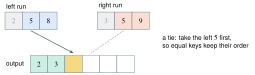
Split a sequence into two smaller sequences, recursively sort each, and merge them. During merging, maintain the invariant that the output contains the smallest already selected elements in sorted order, while the unconsumed parts of both inputs remain sorted. Compare the two next candidates and append the smaller. If they tie, choosing the left candidate preserves the relative order of equal-key records from the original sequence; this is stability.

Correctness follows by induction on length. Length zero or one is already sorted. Assuming the recursive calls return sorted versions of the smaller halves, the merge invariant gives a sorted sequence containing exactly the union of their elements with multiplicity. The halves shrink, so recursion terminates. With linear-time merging, the recurrence is $T(n)=2T(n/2)+\Theta(n)$ in the balanced model, yielding $\Theta(n\log n)$ comparisons/work. The lab allocates output lists and slices, so its space behavior must be analyzed as implemented rather than calling it “in-place.”

Insertion sort is a useful contrast: it maintains a sorted prefix and inserts the next item in the correct position. It is simple and can be efficient on small or nearly sorted inputs, but has quadratic worst-case shifting/comparison cost. Heap sort gives $O(n\log n)$ worst-case time with a different memory/stability tradeoff. Quicksort can have excellent practical behavior, expected $O(n\log n)$ time with appropriate randomization, and quadratic worst case under unsuitable pivots. A standard library’s documented sort should normally be preferred over a classroom reimplementation unless the exercise is to understand the algorithm. [ALGO]

The comparison-sorting lower bound comes from a decision tree: sorting $n$ distinct keys must distinguish $n!$ possible orders. A binary comparison tree needs height at least $\log_2(n!)=\Omega(n\log n)$. Counting sort can avoid that comparison lower bound by using extra assumptions about a bounded integer key universe. Different assumptions mean a different problem model, not a contradiction.

D. Greedy methods need an exchange argument, not confidence#

For selecting the maximum number of nonoverlapping intervals, choosing the earliest-finishing available interval works under the standard unweighted scheduling model. Given an optimal selection, replace its first interval with an earliest-finishing one. This replacement finishes no later and leaves at least as much room for the remaining intervals, so there is an optimal solution beginning with the greedy choice. Repeat on the remaining compatible intervals. The exchange argument is the reason the local rule is globally valid.

A superficially similar greedy rule can fail elsewhere. To make value 6 with denominations $1,3,4$, repeatedly taking the largest possible coin yields $4+1+1$, three coins. The optimum is $3+3$, two coins. “Always take the largest” has no valid general exchange argument for arbitrary coin systems. A few successful examples or familiar real-world denominations do not establish the rule under changed assumptions.

E. Dynamic programming makes dependencies explicit#

Let $D(a)$ be the minimum number of coins needed to make amount $a$, with $D(0)=0$ and unreachable amounts assigned infinity. For positive denominations,

over reachable predecessor amounts. Every optimal nonempty solution has some last coin $d$; removing it leaves an optimal solution for $a-d$, or replacing that remainder with a better one would improve the original. This is optimal substructure. Computing amounts in increasing order is valid because each dependency is smaller.

For denominations $1,3,4$, the table from amount 0 through 6 is $0,1,2,1,1,2,2$. Store a chosen last coin for each reachable amount to reconstruct an actual solution, not merely its count. With $k$ denominations and target $A$, this implementation uses $O(Ak)$ time and $O(A)$ storage. The bound is in the numeric amount $A$, not its bit length $\log A$; this distinction becomes important in complexity theory. Dynamic programming is not automatically a polynomial-time algorithm in the encoded input length.

F. Backtracking explores choices with justified pruning#

Backtracking builds a partial candidate, rejects it as soon as a necessary condition fails, and explores alternatives. For queens on a chessboard, place one queen per row and reject a partial placement sharing a column or diagonal. A four-row solution uses zero-based columns $(1,3,0,2)$. Pruning is sound because adding more queens cannot repair an existing attack between two placed queens. The worst-case search can remain exponential; pruning improves the explored space without changing the need for a correct rejection condition.

Choose a method by structure. Independent smaller subproblems suggest divide and conquer. Repeated overlapping subproblems and an acyclic dependency relation suggest dynamic programming. A provable exchange property may justify greedy choice. Constraint satisfaction without a simpler decomposition may call for backtracking. When the first attempt fails, identify whether it lacks a correct local-choice argument, an adequate state definition, a termination measure, or enough computational resources. Do not replace those questions with algorithm-name guessing.

G. Independent practice#

F foundation C standard course work T transfer S optional stretch L runnable lab or project. Attempt the complete set before opening its solutions.

H. Complete solutions: C07#

Compare the first step where your work differs. A corrected answer is not yet an independent success.

Open every solution

"""C07.05: sorting and exact minimum-coin dynamic programming."""
def merge_sort(values: list[int]) -> list[int]:
    if len(values) < 2:
        return values.copy()
    mid = len(values) // 2
    left, right = merge_sort(values[:mid]), merge_sort(values[mid:])
    out: list[int] = []
    i = j = 0
    while i < len(left) and j < len(right):
        if left[i] <= right[j]:
            out.append(left[i]); i += 1
        else:
            out.append(right[j]); j += 1
    out.extend(left[i:]); out.extend(right[j:])
    return out

def min_coins(coins: list[int], amount: int) -> list[int] | None:
    if type(amount) is not int or amount < 0:
        raise ValueError("nonnegative integer amount required")
    if not coins or any(type(c) is not int or c <= 0 for c in coins):
        raise ValueError("positive integer denominations required")
    best = [amount + 1] * (amount + 1)
    last = [0] * (amount + 1)
    best[0] = 0
    for a in range(1, amount + 1):
        for c in sorted(set(coins)):
            if c <= a and best[a - c] + 1 < best[a]:
                best[a], last[a] = best[a - c] + 1, c
    if best[amount] > amount:
        return None
    out = []
    while amount:
        out.append(last[amount])
        amount -= last[amount]
    return out

if __name__ == "__main__":
    print(merge_sort([4, 1, 3, 1]))
    print(min_coins([1, 3, 4], 6))

I. Retention and readiness#

Retrieve induction, invariants, and amortized versus expected analysis. Advance when you can reject a tempting greedy rule with a counterexample, define a dynamic-programming state precisely, and defend a complexity count without relying on memorized labels.