F19: Performance engineering on a parallel machine: bounds, VLIW packing, SIMD, and batched tree traversal

A. Prerequisites and observable goals#

Level: Frontier track (evidence lane). It is also the foundation for Anthropic’s public performance take-home, a challenge open to any reader (section L). All work uses this chapter’s own toy machine, which is deliberately different from any company’s interview problem.

B. The central idea: every cycle count has two ceilings#

A parallel machine runs one bundle of instructions per clock cycle. Each bundle has a fixed number of slots per engine: so many scalar ALU operations, so many vector operations, so many loads, and so many stores. Our toy machine allows, per cycle:

Every operation takes one cycle, and its result is usable in the next cycle, never the same one. Two things then decide how fast any program can possibly go:

• The critical path. A chain of operations where each needs the previous result cannot finish in fewer cycles than its length. Adding hardware does not help.
• The resource bound. If a program needs $N_e$ operations on engine $e$ with $s_e$ slots, it needs at least $\lceil N_e/s_e\rceil$ cycles. Clever ordering does not help.

The larger of the two is a lower bound: no schedule can beat it. Performance work is a loop of computing that bound, measuring the real count, finding which ceiling you are pressed against, and then changing the program so that ceiling moves. This is the “predict first, simulate second” habit from F01, applied to cycles.

C. Reading a kernel as a dependency graph#

Take $y=(a+b)(c+d)+ef$, with all six inputs loaded from memory and $y$ stored back. Each box below is one operation, and each arrow means “needs the result of”.

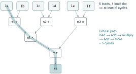
The example as a dependency graph. The longest chain has 5 operations, and the load engine has 6 operations for 1 slot.

The critical path is 5 cycles and the resource bound is $\lceil 6/1\rceil=6$ cycles, so the lower bound is 6. Yet the best schedule takes 9. Bounds are guarantees, not predictions. Here the loads must occupy cycles 0 through 5, and whatever is loaded last still needs three more steps (multiply, add, store) after it arrives. A tighter bound combines the two effects: time to finish the busiest engine, plus the shortest chain that must follow its last operation. Exercise F19.02 walks through it.

D. VLIW packing: filling the slots, cycle by cycle#

A VLIW (very long instruction word) machine has no hardware that reorders your work at run time. The program itself says which operations run together in each cycle. Deciding that is scheduling, and the standard method is list scheduling:

1. Give every operation a height: the length of the longest chain from it to the end of the program.
2. Each cycle, list the ready operations (all inputs finished in earlier cycles).
3. Place them highest-first into any free slot of their engine. Whatever doesn’t fit waits.

Height-first means the operations on long chains start early, so the tail of the program is not left waiting on them.

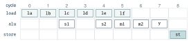
The list schedule on the toy machine. The load engine is full for six cycles; the ALU sits mostly empty. That is what “load-bound” looks like.

Utilization is the fraction of an engine’s slots a schedule fills. Here the load engine is busy $6/9$ of the time and the four ALU slots only $5/36$. When one engine sits near 100% and the others are nearly idle, that engine is the bottleneck. Removing its work is the only way to go faster.

E. Independent work: why one chain wastes the machine#

A single chain of 6 dependent vector operations takes 6 cycles no matter how many vector slots exist, because each operation waits for the last. With 2 slots, half the vector engine sits idle. Two independent chains, such as two iterations of a loop that don’t depend on each other, interleave perfectly: still 6 cycles, but twice the work and 100% utilization. With 8 chains ($48$ operations), the resource bound takes over: $\lceil48/2\rceil=24$ cycles.

This is the logic behind loop unrolling. Copy the loop body so several independent iterations are in flight at once, and the scheduler always has something ready to run. The lab’s independent_chains function and its utilization report let you watch the switch from latency-bound to resource-bound happen.

F. SIMD: one instruction, many lanes#

A vector instruction applies one operation to every lane of a vector at once. The toy machine has 4 lanes.

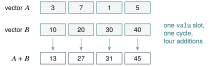
Adding 1,000 pairs takes 1,000 scalar additions, which is 250 cycles on 4 ALU slots. As vectors it takes $1000/4=250$ vector additions, which is 125 cycles on 2 vector slots. SIMD pays when every lane does the same operation on data arranged side by side in memory (a structure of arrays). Two things break it:

• Tails. 1,002 elements need 251 vectors; the last is only half full, so you mask it or finish it with scalar operations.
• Different addresses per lane. A contiguous vector load fetches 4 neighbours in one operation. If each lane needs a value from a different place (a gather), a machine without a gather instruction must issue one scalar load per lane. Now the load engine, not the vector engine, sets the pace. This is exactly what happens in tree traversal.

G. Scratch memory: the data you keep close#

CPUs cache recently used data automatically. Many accelerators instead give you a small scratchpad and make you decide what lives there. That makes it a budget: every word kept resident is a load you never repeat, and every word costs space. Two questions guide every scratchpad decision:

1. Is this value reused? Loading something once and using it many times from scratch turns repeated loads into free reads.
2. What does keeping it cost? Space, plus any extra arithmetic needed to pick the right resident value, can outweigh the loads saved. Section I puts numbers on this trade-off.

H. Hiding latency: software pipelining#

Suppose each loop iteration loads a value, does two dependent vector operations, and stores the result: four steps in a chain. Run iterations one at a time and $N$ iterations cost $4N$ cycles. But iteration 2’s load doesn’t depend on iteration 1’s arithmetic. Start it one cycle later and the iterations overlap like an assembly line:

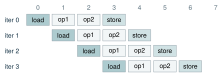
Software pipelining: once the pipe is full, one iteration finishes every cycle. Each cycle uses 1 load, 2 vector operations, and 1 store, exactly the toy machine’s limits.

After a short start-up, one iteration completes per cycle, so $N$ iterations take about $N+3$ cycles instead of $4N$. The limit is again a resource: one load slot and one store slot allow at most one iteration per cycle. Software pipelining is what unrolling becomes when you plan the overlap deliberately.

I. Case study: batched traversal of a binary search tree#

Now a real kernel. You have a sorted table of keys and a batch of queries: for each query, how many keys are smaller? (This is the heart of decision-tree inference, database indexes, and many lookups in engines.)

Step 1: put the tree in an array. The Eytzinger layout stores a complete binary search tree with the root at index 1 and the children of node $i$ at $2i$ and $2i+1$. There are no pointers, just arithmetic. For the 15 keys $1,2,\ldots,15$:

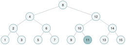
index	1	2	3	4	5	6	7	8	9	10	11	12	13	14	15
key	8	4	12	2	6	10	14	1	3	5	7	9	11	13	15

The same tree, drawn and stored. Walking the drawing left to right reads the keys in sorted order.

Step 2: search without branches. Start at $i=1$. At each level, go right exactly when the query is larger than the node:

where $[\,\cdot\,]$ is 1 if true and 0 if false. After $D$ levels, the path has spelled the answer in binary: $\text{rank}=i-2^D$. For $q=11$: $i=1\to3\to6\to13\to26$, so the rank is $26-16=10$, and indeed ten keys ($1$ to $10$) are smaller. There is no if: the comparison result is the arithmetic. That matters because a vector lane cannot take its own branch, but it can add a 0 or a 1.

Step 3: move the whole batch in lockstep. Every query takes exactly $D$ steps, so process level by level: all queries do level 0, then all do level 1, and so on. Each lane of a vector carries one query. The work per level per vector is one compare and one index update, which is regular, independent, and schedulable.

Step 4: find the bottleneck. The index update is cheap. The expensive part is fetching $\text{tree}[i]$, because every lane’s $i$ is different, so every lane needs its own load. With 256 queries and 10 levels, that is $2{,}560$ scalar loads on 1 load slot: at least $2{,}560$ cycles, while the vector engine needs only $64\times2\times10=1{,}280$ operations (640 cycles). The kernel is load-bound.

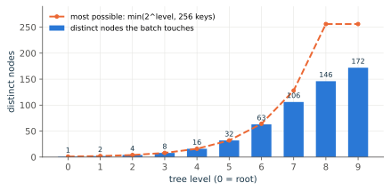
Step 5: keep the top of the tree resident. Level $\ell$ has only $2^\ell$ nodes, so the top few levels are tiny and every query passes through them. Load them once into scratch memory and stop loading them per query. The price is that each lane must now select its node value from the resident candidates, which costs $2^\ell-1$ vector selects per vector at level $\ell$. Loads fall linearly while selects grow exponentially, so there is a best number of levels to cache:

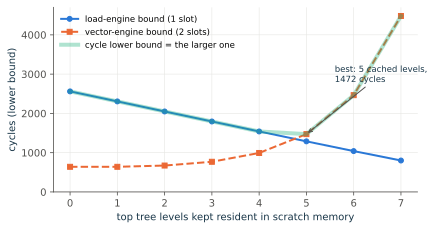
This is the whole method in one picture: find the busiest engine, move work off it, and stop when another engine becomes the bottleneck. The model is simple on purpose. Real kernels add hashing, wrap-arounds, tails, and scheduling limits, but each of those changes the operation counts, not the reasoning.

J. Working like a performance engineer#

• Bound before you touch code. Count operations per engine and the longest chain. Write the lower bound at the top of your log.
• Build tools early. A per-engine utilization report takes about 30 lines and tells you which ceiling you are pressed against. Anthropic has written that how candidates invest in tooling is part of what its take-homes measure.
• One change, one measurement. Keep a log with columns for change, cycles, delta, which bound moved, and whether the tests pass. It becomes your write-up and the story you tell in a design review or an interview.
• Correctness is non-negotiable. Re-run the full correctness check after every change. A faster wrong answer is not an optimization.

K. The lab#

The lab ships with its starters and tests in the companion code’s frontier_code folder (bezhig.com/book), and needs only Python’s standard library. starters/perf_lab.py has three blanks: critical_path (F19.L1), list_schedule (F19.L2), and search_batch_lockstep (F19.L3). Everything else (graph checking, heights, the schedule verifier, utilization, the Eytzinger builder, and the cost model) is provided for you to read and use.

cd frontier_code
$env:MANUAL_IMPL = "starters"          # PowerShell
python -m unittest tests.test_perf -v
python verify_f19.py                   # the numbers quoted in this chapter

In bash or zsh, set the variable with export MANUAL_IMPL=starters instead.

L. A public challenge: Anthropic’s performance take-home#

Anthropic open-sourced its original performance-engineering take-home, and in January 2026 it told the story of the test. It is a simulated accelerator with VLIW bundles, SIMD vector operations, and a scratchpad you manage by hand, running a batched tree-traversal kernel scored in cycles. The first version, used from early 2024, gave candidates 4 hours and a multicore machine; version 2 cut it to 2 hours without multicore; Anthropic retired version 2 after Claude Opus 4.5 matched the best human 2-hour score. The public repository is therefore a showcase, not practice for the live screen. It invites an email for a solution under 1,487 cycles, warns that new models may move that bar, and accepts a result only if the tests/ folder is unchanged. The live test, as of January 2026, is a set of puzzles on a constrained instruction set, scored by instruction count, with only a validity checker supplied: no debugger, so you build your own tools, and how you invest in them is part of what is measured. Everything in sections B–J transfers directly. The machine, the kernel, and the numbers do not, and working them out is the challenge.

1. Recon (one session, before studying). Clone the repository, run its submission test, record the starting cycle count, and read the README and the simulator code until you can say what one bundle may contain. Write down three things you don’t understand. Don’t optimize yet; the goal is to make this chapter’s ideas feel necessary.
2. Foundations. Read C09 on instructions and caches, then T01 on finding the limiting resource, and the roofline section of G06. Then work this chapter and pass all 19 lab tests on your own starter code.
3. Bound the real kernel. Using the simulator’s slot limits, count operations per engine for the reference kernel and compute its lower bound by hand. Compare it with the measured baseline.
4. Tooling, as the live test demands. Build a per-engine utilization report for the simulator’s traces before your first optimization. Then the drill that matches the live test as Anthropic described it in January 2026: invent a tiny instruction set of your own (five or six instructions and a few registers), write a tracer that prints machine state after each instruction, and solve three puzzles of your own design for the fewest instructions, using only a checker that says valid or invalid.
5. Timed attempts. Do one 2-hour attempt first, the time version 2 allowed, and log every change. Expect it to be harder than version 2 was: this repository restores the slowest starting kernel, while version 2 began from a kernel about 8 times faster. Then continue with unlimited time. Re-run the correctness tests after every change.
6. Validate like a reviewer. None of the public submissions under 1,300 cycles in the repository’s first day were valid: language models had edited the tests. Keep a clean clone, confirm that git diff origin/main tests/ prints nothing, and run python tests/submission_tests.py before you believe any number.
7. Write it up. Your log becomes a short, honest write-up: what bounded the kernel at each stage, what moved it, and the command that reproduces the final count.

Sources for this section (checked 17 October 2026)#

• Anthropic Engineering, on designing technical evaluations that resist AI (January 2026), the history of the take-home and the live test’s format: www.anthropic.com/engineering/AI-resistant-technical-evaluations.
• The repository, its README, the 1,487-cycle invitation, and its validation steps: github.com/anthropics/original_performance_takehome.
• Anthropic’s candidate guidance on AI use (updated 10 July 2025): www.anthropic.com/candidate-ai-guidance.

M. Independent practice#

F foundation C standard course work T transfer S optional stretch L runnable lab or project. Attempt the complete set before opening its solutions.

N. Complete solutions: F19#

Compare the first step where your work differs. A corrected answer is not yet an independent success.

Open every solution

O. Retention and readiness#

Without notes, compute the two bounds for a kernel you invent with 8 loads and a 4-step chain, then explain aloud why caching tree levels eventually stops paying. Revisit F19.02 and F19.07 in a week. Log misses under the error families in LM (Part I); “counting” slips go under bookkeeping.