G05: Numerical linear algebra and optimization

Prerequisites and observable goals#

The central question: which problem is hard, and which algorithm is fragile?#

A poorly conditioned problem changes its answer substantially when its data changes slightly. An unstable algorithm can introduce unnecessary error even on a well-conditioned problem. These are not synonyms. Report the norm, perturbation model, and object whose error is measured before calling a calculation “accurate.”

For an invertible matrix $A$, the normwise condition number in the Euclidean norm is $\kappa_2(A)=\|A\|_2\|A^{-1}\|_2=\sigma_{\max}/\sigma_{\min}$. A small singular value means some input direction produces a small output: recovering its coefficient from noisy observations is difficult. Adding more decimal digits to printed output does not solve that loss of information.

Least squares is geometry with a residual#

For $A\in\R^{m\times n}$ and $b\in\R^m$, minimize

When $A$ has full column rank, the minimizer is unique. Differentiation gives $\nabla F(x)=A^T(Ax-b)$; at the minimizer, the residual $r=Ax-b$ is orthogonal to every column of $A$:

These normal equations characterize the optimum, but explicitly forming them is not always a good numerical algorithm. Their condition number satisfies $\kappa_2(A^TA)=\kappa_2(A)^2$ under full column rank, potentially magnifying numerical difficulties.

Worked example: fit a line $a+bt$ to $(t,y)=(0,1),(1,2),(2,2)$. Then

The equations $3a+3b=5$ and $3a+5b=6$ give $b=1/2$, then $a=7/6$. Predictions are $(7/6,5/3,13/6)$, so $r=(1/6,-1/3,1/6)$. Check $\sum_i r_i=0$ and $\sum_i t_ir_i=0$. The squared residual norm is $1/6$, hence the half-squared objective is $1/12$. These checks make the geometry visible.

Orthogonal transformations preserve distances#

An orthogonal matrix $Q$ satisfies $Q^TQ=I$, so $\|Q^Tv\|_2=\|v\|_2$. A thin QR factorization of full-column-rank $A$ writes $A=Q_1R$ with $Q_1$ having orthonormal columns and $R$ upper triangular. Completing to an orthogonal basis gives

Only the first term depends on $x$. Solve the triangular system $Rx=Q_1^Tb$ by back substitution; the leftover component is the irreducible residual. The algorithm avoids explicitly squaring the condition number by forming $A^TA$.

A Householder step, derived#

Given a nonzero column segment $z$, we want a reflection that maps it to a multiple of the first coordinate vector $e_1$. Choose $\alpha=-\operatorname{sign}(z_1)\|z\|_2$ (choose positive sign for a zero $z_1$), set $v=z-\alpha e_1$, and define

Since $P=vv^T/(v^Tv)$ is an orthogonal projector with $P^2=P$, $H^TH=(I-2P)^2=I$. One can check $Hz=\alpha e_1$. The sign choice avoids subtracting nearly equal positive quantities when constructing the first component of $v$.

For $z=(3,4)^T$, choose $\alpha=-5$ and $v=(8,4)^T$. Then

The reflection changes orientation but not length. Apply it to the active rows of each remaining matrix column and to the matching target segment. Repeat down the diagonal. The lab stores and applies each reflector directly rather than constructing a dense $H$ each time.

What the reference does and does not promise#

The implementation globally scales $A$ and $b$ by the largest absolute matrix entry, computes Householder steps with math.hypot, and rejects a sufficiently small remaining diagonal segment using a documented relative threshold. This is an educational full-rank solver, not a rank-revealing pivoted QR or SVD library. A tolerance-based rank decision depends on scaling and column order. Very ill-conditioned or extreme dynamic-range cases require stronger tools, condition estimates, and careful residual/backward-error analysis.

A small residual is not always a small coefficient error: with nearly dependent columns, many widely different coefficients predict almost the same vector. Conversely, a nonzero residual can be unavoidable for noisy or inconsistent observations, even when the computed minimizer is excellent. To check a result, report both residual size and sensitivity, not one scalar relabeled as universal accuracy.

Gradient descent on a quadratic#

Let $f(x)=\frac12x^THx-g^Tx$ with symmetric positive-definite $H$. The optimum solves $Hx_*=g$. Gradient descent uses

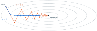
where $e_k=x_k-x_*$. In an orthonormal eigenbasis of $H$, each error component is multiplied by $1-\eta\lambda_i$. All shrink in magnitude when

At the endpoint, the largest-eigenvalue component can oscillate without decay. A tiny step is stable but can be slow, especially when $\lambda_{\max}/\lambda_{\min}$ is large. The formula derives from this quadratic model; do not apply it to an arbitrary neural-network loss without establishing relevant smoothness and curvature assumptions.

For $H=\diag(1,9)$ and $g=0$, choosing $\eta=.1$ yields factors $.9,.1$. Starting $(1,1)$ gives $(.9,.1)$ and objective $(.81+9(.01))/2=.45$, down from 5. Choosing $\eta=.3$ yields factors $.7,-1.7$; the second component grows while changing sign. A decreasing loss in one tested step does not prove global convergence on a different objective.

Constraints and first-order conditions#

For differentiable convex $f$, a zero gradient is a global minimum on all of $\R^n$. With constraints, zero gradient need not hold at the constrained optimum. For $\min_x (x-2)^2$ subject to $x\le1$, the optimum is 1, whose derivative is $-2$. Using $g(x)=x-1\le0$, the Lagrangian is $\mathcal L=(x-2)^2+\lambda(x-1)$. At the optimum, stationarity gives $-2+\lambda=0$, so $\lambda=2\ge0$ and complementary slackness $\lambda g(x)=0$ holds. General KKT necessity needs a suitable constraint qualification; sufficiency in convex settings needs the appropriate convexity and feasible conditions. This example does not establish KKT for every nonconvex program. [G-CVX]

Independent practice#

F foundation C standard course work T transfer S optional stretch L runnable lab or project. Attempt the complete set before opening its solutions.

Smallest useful hints#

For .02, write $v=(8,4)$ and compute its outer product before division. For .03, solve each diagonal equation separately. For .06, transform the target using exactly the same row reflection as the matrix.

Complete solutions: G05#

Compare the first step where your work differs. A corrected answer is not yet an independent success.

Open every solution

"""G05: educational Householder least squares for bounded full-rank matrices."""
import math


def least_squares(A, b, rtol=1e-12):
    m, n = len(A), len(A[0]) if A else 0
    if not 1 <= n <= 64 or not n <= m <= 10000 or len(b) != m:
        raise ValueError("require m >= n, 1..64 columns, <=10000 rows")
    if any(len(row) != n for row in A):
        raise ValueError("ragged matrix")
    if not math.isfinite(rtol) or not 0 < rtol < 1:
        raise ValueError("relative rank threshold must lie in (0,1)")
    if any(not math.isfinite(x) for row in A for x in row) or any(not math.isfinite(x) for x in b):
        raise ValueError("finite matrix and target required")
    scale = max(abs(x) for row in A for x in row)
    if scale == 0:
        raise ValueError("rank-deficient zero matrix")
    R = [[x/scale for x in row] for row in A]
    target = [x/scale for x in b]
    if any(not math.isfinite(x) for x in target):
        raise ValueError("target exceeds supported dynamic range")
    for j in range(n):
        z = [R[i][j] for i in range(j,m)]
        norm = math.hypot(*z)
        if norm <= rtol:
            raise ValueError("rank deficiency at stated relative threshold")
        alpha = -math.copysign(norm,z[0])
        v = list(z)
        v[0] -= alpha
        vnorm = math.hypot(*v)
        v = [x/vnorm for x in v]
        for k in range(j,n):
            projection = 2*math.fsum(v[i-j]*R[i][k] for i in range(j,m))
            for i in range(j,m):
                R[i][k] -= projection*v[i-j]
        projection = 2*math.fsum(v[i-j]*target[i] for i in range(j,m))
        for i in range(j,m):
            target[i] -= projection*v[i-j]
        R[j][j] = alpha
        for i in range(j+1,m):
            R[i][j] = 0.
    x = [0.]*n
    for j in range(n-1,-1,-1):
        remainder = math.fsum(R[j][k]*x[k] for k in range(j+1,n))
        x[j] = (target[j]-remainder)/R[j][j]
    if not all(math.isfinite(value) for value in x):
        raise ValueError("nonfinite coefficients")
    return x


if __name__ == "__main__":
    print(least_squares([[1,0],[1,1],[1,2]],[1,2,2]))

Readiness and continuation#

Explain why an inconsistent system has a best approximation, why $A^Tr=0$ is geometric, and why a small residual need not mean stable coefficients. Continue with pivoted QR, SVD-based rank determination, backward stability proofs, preconditioning, iterative Krylov solvers, and constrained convex optimization. The optional reference gives deeper convex analysis; only its public book page was used as a continuation pointer here. [G-CVX]