A01: Linear systems, vector spaces, and transformations

A. Prerequisites and observable goals#

Level: Degree-core mathematics; no calculus prerequisite.

B. The central question: which combinations produce the desired output?#

A vector is an ordered collection of coordinates relative to a chosen basis. It can describe displacement, a feature representation, a sampled signal, or a collection of unknowns. The same tuple can have different meanings in different coordinate systems. Addition and scalar multiplication are coordinatewise: $(1,2)+(3,-1)=(4,1)$ and $2(1,2)=(2,4)$. A linear combination is a sum $c_1v_1+\cdots+c_kv_k$. The coefficients $c_i$ are scalars; the $v_i$ are vectors. Do not confuse the number of coefficients with the dimension of each vector.

A matrix $A\in\R^{m\times n}$ is a rectangular array with $m$ rows and $n$ columns. It represents a linear map from $\R^n$ to $\R^m$. Writing its columns as $a_1,\dots,a_n$ makes multiplication meaningful:

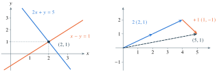
Thus $Ax=b$ asks whether the desired output $b$ can be assembled from the columns of $A$, and, if so, with which coefficients. This connects an algebraic system with a geometric image rather than treating multiplication as a mysterious row-by-column ritual.

C. Span, independence, and bases#

The span of a collection is the set of all its linear combinations. A collection is linearly independent when the only coefficients producing the zero vector are all zero. A basis for a vector space is an independent spanning collection; its size is the dimension. For example, $(1,0)$ and $(0,1)$ form a basis of $\R^2$. So do $(1,1)$ and $(1,-1)$. The coordinates of a vector change with the basis, while the represented geometric vector need not.

The null space $\ker A=\{x:Ax=0\}$ describes inputs collapsed to zero. The column space $\operatorname{im} A=\{Ax:x\in\R^n\}$ describes achievable outputs. The rank is the dimension of the image. The rank–nullity theorem states

where $n$ is the dimension of the input space. One way to understand this is to extend a basis of the null space to a basis of the whole input space. The added basis vectors have images that form a basis of the image: they must span it, and any dependence would contradict the way the original basis was completed. Each lost input direction reduces the number of independent output directions.

D. Elimination preserves the solution set#

Consider

Add the equations to obtain $3x=6$, so $x=2$; substitute into $x-y=1$ to obtain $y=1$. The augmented matrix records the same operations:

Swapping equations, multiplying an equation by a nonzero scalar, and adding a multiple of one equation to another are reversible operations. They preserve exactly the same solutions. Multiplying a row by zero is not reversible and can erase a constraint. A pivot is a leading nonzero entry used to eliminate a variable from other equations. If a prospective pivot is zero, exchange rows when possible; do not divide by zero and hope a later simplification repairs it.

A row $[0\ 0\mid 1]$ means $0=1$: the system is inconsistent. A row of all zeros means one constraint is redundant. A nonpivot input variable is free in a consistent system. For example,

has $(x,y)=(3-2t,t)$ for every real $t$, not merely one numerical answer. Changing the second right-hand side to 7 makes the system inconsistent. The coefficient matrix has rank 1 in both cases, but the right-hand side changes consistency.

E. Composition explains matrix multiplication#

Suppose $B:\R^p\to\R^n$ and $A:\R^n\to\R^m$. The composition $x\mapsto A(Bx)$ has matrix $AB\in\R^{m\times p}$. Column $j$ of $AB$ is $A$ applied to column $j$ of $B$. Dimensions enforce which multiplication is meaningful; the order follows the function composition. In general $AB\ne BA$, even when both products exist.

A planar rotation and nonuniform scaling demonstrate the difference. With

$RS(1,0)^T=(0,2)^T$, whereas $SR(1,0)^T=(0,1)^T$. Applying local scale before world rotation is not the same as scaling along world axes afterward. Translation $x\mapsto Ax+t$ is affine, not linear when $t\ne0$, because it does not send zero to zero. Homogeneous coordinates encode an affine map in a larger matrix, but they do not make the original translation a linear map on the original vector space.

F. Inverses and determinants: useful but not universal tools#

For a square matrix, invertibility, full rank, trivial null space, independent columns, and nonzero determinant are equivalent. The inverse undoes the map. To solve one numerical system, elimination or a factorization is generally preferable to explicitly forming an inverse: the inverse computes more information than the requested solution and can introduce avoidable work or error. [LA]

In two dimensions, $\det\begin{pmatrix}a&b\\c&d\end{pmatrix}=ad-bc$ is an oriented area scale factor. Its absolute value describes area scaling; its sign distinguishes orientation preservation from reversal. A zero determinant identifies dimension collapse. It is not a general measure of numerical quality: $\operatorname{diag}(10^{12},10^{-12})$ has determinant 1 but stretches different directions by vastly different amounts. Conditioning in A05 and singular values in A02 explain that problem more accurately.

G. Independent practice#

F foundation C standard course work T transfer S optional stretch L runnable lab or project. Attempt the complete set before opening its solutions.

H. Complete solutions: A01#

Compare the first step where your work differs. A corrected answer is not yet an independent success.

Open every solution

"""A01.05: exact Gaussian elimination on small rational systems."""
from fractions import Fraction

def solve_exact(a: list[list], b: list) -> list[Fraction]:
    n = len(a)
    if n == 0 or len(b) != n or any(len(row) != n for row in a):
        raise ValueError("nonempty square system required")
    m = [[Fraction(v) for v in row] + [Fraction(rhs)]
         for row, rhs in zip(a, b)]
    for k in range(n):
        pivot = next((i for i in range(k, n) if m[i][k] != 0), None)
        if pivot is None:
            raise ValueError("system is not uniquely solvable")
        m[k], m[pivot] = m[pivot], m[k]
        for i in range(k + 1, n):
            factor = m[i][k] / m[k][k]
            for j in range(k, n + 1):
                m[i][j] -= factor * m[k][j]
    x = [Fraction(0)] * n
    for i in range(n - 1, -1, -1):
        x[i] = (m[i][n] - sum(m[i][j] * x[j]
                             for j in range(i + 1, n))) / m[i][i]
    return x

if __name__ == "__main__":
    print(solve_exact([[2, 1], [1, -1]], [5, 1]))

I. Retention and readiness#

Retrieve function composition from Module 03 and the difference between a factor and an additive term from Module 01. Advance when you can explain $Ax=b$ both as equations and as a column combination, and can recognize a free variable without treating it as a missing calculation.