Module 13: Linear approximation, extrema, and the Mean Value Theorem
On this page
- A. Prerequisites and observable goals
- B. The central idea: local slopes constrain global change
- C. Three different statements
- D. Why these conclusions make sense
- E. Choose the question before choosing the theorem
- F. Worked teaching examples
- F1. Over or under? Concavity, borrowed from Module 14
- F2. Differentials: how a measurement error travels
- F3. Three traps and a faded example
- G. Independent practice
- Drill set: the friction points
- Frontier applications
- A robot’s position filter
- Hint ladders for M13.09–M13.22
- H. Complete solutions: Module 13
- Spaced review answers
- Faded example answer
- I. Retention and readiness
A. Prerequisites and observable goals#
Tangent lines, derivative rules, continuity, and interval notation.
Estimate a nearby value with a tangent line, identify candidate extrema, and use the Mean Value Theorem with its hypotheses intact.
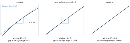
Picture 13.1. Zoom in until the curve is a line. Three views of (black) and its tangent line at (blue, dashed). The vertical axis is stretched six times so that the bend shows, and each zoom multiplies both scales by . At the widest view the curve visibly bends below the line. Each zoom shrinks the gap at the window’s edge about to times, close to and far more than : for a smooth curve like this one, whose second derivative exists, the tangent line’s error shrinks like the square of the step (Module 30 makes this exact: about ). Differentiability alone promises less, only that the error shrinks faster than the step. Either way, is an excellent estimate close to and a poor one far away.
B. The central idea: local slopes constrain global change#
A derivative is local: it describes change near one input. A tangent line turns that information into a nearby approximation. The Mean Value Theorem (MVT) connects local slopes to an average slope over an entire interval. Extrema ask where a function becomes largest or smallest; derivatives help locate candidates but do not replace comparison of their values.
C. Three different statements#
The linearization of a differentiable function at is the exact affine function
The statement is an approximation. More precisely, differentiability means : the error divided by tends to zero. This is not a promise that an arbitrary step such as is small enough.
The Extreme Value Theorem (EVT) says that a continuous real function on a closed bounded interval attains an absolute maximum and an absolute minimum. A critical number is an interior domain input where or does not exist. An interior local extremum of a differentiable function has derivative zero (Fermat’s theorem); the converse is false.
The Mean Value Theorem assumes continuity on and differentiability on , with . It guarantees at least one such that
Rolle’s theorem is the special case , which gives . The theorem guarantees existence, not a unique or a method for finding it in every problem. Definitions and hypotheses: [O1MVT].
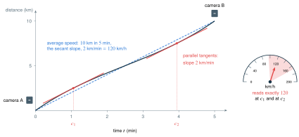
Picture 13.2. The speed trap. Two cameras km apart log a car minutes apart, so its average speed is km/h, the slope of the blue secant. The car passed camera A at km/h, slowed to km/h, and sped back up to km/h at camera B (the shaded arc on the dial is that range). Whatever happened in between, the Mean Value Theorem guarantees a moment when the speedometer read exactly : a tangent parallel to the secant. Here there are two such moments. A ticket based on average speed is a theorem, not a guess.
D. Why these conclusions make sense#
For a differentiable local maximum at , sufficiently small positive increments give , while negative increments give a quotient . If the common finite limit exists, it must be zero. This argument fails at an endpoint because one of the two directions may be unavailable.
To see the MVT, subtract the secant line from . The new function has equal endpoint values. Rolle’s theorem supplies a horizontal tangent to that difference, meaning that has a tangent parallel to its secant. Rolle’s theorem follows from the EVT: either the function is constant or a maximum or minimum occurs in the interior, where Fermat’s theorem applies. Each hypothesis has a job: endpoints secure extrema, continuity prevents jumps, and differentiability excludes corners at the crucial interior extremum.
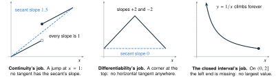
Picture 13.3. Every hypothesis has a job. Remove one hypothesis and the conclusion can fail. Left: without continuity, the Mean Value Theorem fails. Middle: without differentiability, Rolle’s theorem fails. Right: without a closed interval, the Extreme Value Theorem fails. A failed hypothesis means the theorem is silent, not that its conclusion must be false.
E. Choose the question before choosing the theorem#
For a nearby estimate, choose a convenient base point with known and . For absolute extrema on , confirm continuity, find all interior critical numbers, and compare their function values with both endpoints. For an existence or rate-bound question, inspect the MVT hypotheses first. An unavailable hypothesis means the theorem cannot justify the conclusion; it does not automatically mean the conclusion is false.
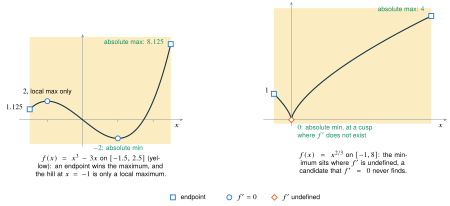
Picture 13.4. Every candidate gets a vote. The closed-interval method in pictures. List three kinds of candidates: both endpoints (squares), every interior with (circles), and every interior where does not exist (diamond). Then compare their heights: the largest is the absolute maximum and the smallest the absolute minimum. Skip a kind of candidate and you can miss the answer.
F. Worked teaching examples#
Estimating a square root. Let , and use because . Then and
Since for , the graph is concave down and its tangent lies above it; the estimate is an overestimate. The value is exact for , not for the square root.
An MVT calculation. For on , the average slope is . Solving gives , which is inside the open interval. Checking location is part of using the theorem.
Finish the candidate list. For on , . Before calculating values, list the four inputs that must be checked. They are , not just the two derivative zeros. Their heights are ; both absolute extrema occur more than once.
F1. Over or under? Concavity, borrowed from Module 14#
Every linearization in this module ends with the question “too high or too low?” The answer comes from the way the graph bends. Module 14 develops bending fully; here is the one fact you need now, proved with this module’s own theorem.
Picture 13.1 shows the fact at work: has , so the curve stays under its tangent, and is a little too high.
F2. Differentials: how a measurement error travels#
Linearization has a second job. Besides estimating a value, it predicts how an error in an input becomes an error in an output. Call a small change in the input , and call the tangent line’s change :
The true change is close to when is small; Picture 13.1 shows how close. Engineers use this line to build error budgets: how precisely must each part be measured for the result to be good enough?
Worked example. A cube’s edge is measured as cm, possibly off by cm either way. Its volume is , so
The volume is cm, possibly off by about cm. As fractions of the whole, the edge is off by and the volume by : three times as much.
The exponent multiplies the relative error. For any power law ,

The cube’s exponent is , so its edge error becomes a volume error. A square root () halves a relative error, and a cube triples it. High exponents are where precision matters: in slow, smooth (laminar) pipe flow under a fixed pressure drop, the flow rate grows like the fourth power of the radius (Poiseuille’s law), so a error in a pipe’s radius becomes a error in its predicted flow.
F3. Three traps and a faded example#
G. Independent practice#
F foundation C standard course work T transfer S optional stretch L runnable lab or project. Attempt the complete set before opening its solutions.
Use linearization to estimate . State the base point and distinguish the estimate from an exact value.
Use at to estimate . Decide whether the tangent estimate is above or below the true value.
Find the absolute extrema of on .
Find every MVT point for on .
Why does Rolle’s theorem not apply to on ? Show directly that its conclusion fails.
Suppose is continuous on , differentiable on , , and . Bound .
Give a differentiable function whose derivative is zero at an input that is not a local extremum. Give a continuous function on with neither an attained maximum nor an attained minimum.
Use the MVT to prove for all real . Explain what this says about input error.
Drill set: the friction points#
Each problem names the friction family it trains. Do them in order: they get less familiar as they go. Hint ladders follow the original hints.
(Fractions under pressure; a root in disguise.) Linearize at and use it to estimate . Is the estimate too high or too low?
(Bookkeeping: negative exponents.) Linearize at and use it to estimate . Too high or too low?
(Angle Fortress; small angles.) Linearize and at . Use them to estimate and , compare with a calculator, and use concavity to explain why the cosine estimate has the larger error.
(Derivative on top.) Linearize at and at . Estimate and , and decide whether each estimate is too high or too low.
(Differentials.) A sphere’s radius is measured as cm, possibly off by cm. Estimate the largest possible error in its computed volume, and the relative error.
(An error budget.) For small swings, a pendulum of length has period . If its length is measured with a relative error, estimate the relative error in . How precisely must be measured for to be good to ?
(The forgotten candidates; fractions.) Find the absolute extrema of on .
(Angle Fortress.) Find the absolute extrema of on .
(The Mean Value Theorem with a root.) Check the Mean Value Theorem’s hypotheses for on , then find every it promises.
(The Mean Value Theorem as a bound.) Use the Mean Value Theorem on to prove, without a calculator, that .
(Rolle: exactly one root.) Show that has exactly one real solution, and that it lies between and .
Frontier applications#
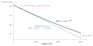
Picture 13.5. A barometer’s straight-line model. Pressure (black) is concave up, so its tangent line at the ground (blue, dashed) lies below it everywhere else. Near the ground the line is excellent; by km it is off by kPa, about m of altitude.
The altimeter in your drone. (a) Linearize at and give the slope in pascals per metre. Check it against the hydrostatic rule , with kg/m and m/s. (b) In flight, the reading has dropped Pa since takeoff. Estimate the altitude. (c) If the pressure reading jitters by Pa, how much does the altitude estimate jitter? (d) At a true altitude of m, find the exact pressure, then the altitude the straight-line model would report from it. Is the line too high or too low, and is it good enough for a m flight?
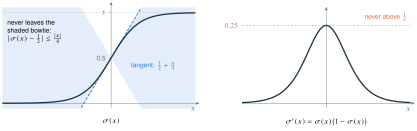
Picture 13.6. The sigmoid’s speed limit. Left: and its tangent line at . Right: its slope, which is never more than . By the Mean Value Theorem, that slope limit becomes a global promise: from the point the curve stays inside the shaded bowtie of slopes , which beyond already covers the whole strip between and . In a real network each layer also multiplies by its weights, so this limit does not force learning signals to fade; with weights of modest size, fading is the typical case.
Why deep sigmoid networks learn slowly. (a) Show that . (b) Linearize at and estimate . Is the estimate too high or too low, and why? (c) Show that for every , and use the Mean Value Theorem to prove for all and . (d) A signal passes through a chain of sigmoids, each one’s output the next one’s input, with no weights in between: , , and so on to . By the chain rule, how large can possibly be? A real network also multiplies by a weight at every layer; in one sentence, explain why this fading still helped push modern networks toward activations such as ReLU, whose slope is exactly for positive inputs.
A robot’s position filter#
A sidewalk delivery robot drives at walking pace and reports its position to a tracking computer twenty-five times a second. Position fixes are slightly noisy, and now and then one is wildly wrong. The tracker keeps the last position it accepted and discards any report that lies farther away than the robot could have driven since then, plus a fixed allowance:
float dist    = distance(lastAccepted, reported);   // cm
float maxDist = MAX_SPEED * speedFactor * gap;      // cm

if (dist > maxDist + TOLERANCE) {
    // a glitch: discard the report and keep lastAccepted
} else {
    lastAccepted = reported;
}
Here MAX_SPEED is cm/s, TOLERANCE is cm, and speedFactor is unless a setting raises the robot’s top speed. The time gap starts from the gap on the tracker’s own clock since the previous report. That clock is a tick count: it moves in steps of s, twenty-five times a second. When a report carries the robot’s own timestamp, later than its previous one, the gap is raised to the robot’s own gap, capped at s; and the result is never less than s.
(The Mean Value Theorem as a glitch filter.) Take speedFactor unless told otherwise, so the speed cap is cm/s. (a) The robot drives along any path at a speed that never exceeds . Let be the distance driven along the path by time , so is the speed. Use the Mean Value Theorem on to show that between two reports apart the straight-line jump dist is at most , so the filter never discards an accurate report, provided gap is at least the true . (b) A report claims a cm jump s after the previous one. Is it discarded? If the jump had been real, what does the Mean Value Theorem say about the robot’s speed at some instant? (c) Network delay bunches two reports that were sent s apart, so the tracker handles both in the same tick. What maxDist does the tracker use if the reports carry no timestamps, and if they do? Why does a genuine cm step pass either way? What job does the cm tolerance do? (d) A software update raises the robot’s top speed by , so speedFactor becomes . How long a gap makes the cm jump acceptable?
Optional small hints
For M13.03, endpoints are candidates too. For M13.06, the MVT places the average slope between the derivative bounds. For M13.08, use the derivative of sine and .
Hint ladders for M13.09–M13.22#
Climb one rung at a time, and try the problem again after each rung.
Rung 1: a nudge
Which nearby input has a power you can do in your head?
Rung 2: the idea
The linearization ; top minus bottom over bottom for .
Rung 3: a skeleton
, ; ; the sign of decides over or under.
Rung 1: a nudge
What does look like with no fraction bar?
Rung 2: the idea
Parentheses Rewrite, then the power rule; watch the exponent’s sign.
Rung 3: a skeleton
, ; ; , so the graph is concave .
Rung 1: a nudge
What are , , and their slopes?
Rung 2: the idea
Each linearization is . The error depends on how much the graph bends at , which is .
Rung 3: a skeleton
and ; compare with .
Rung 1: a nudge
What are and , and their slopes?
Rung 2: the idea
Derivative on top, original on bottom: . Concavity decides over or under.
Rung 3: a skeleton
near ; near ; is concave and is concave .
Rung 1: a nudge
Which formula links radius and volume, and what is its derivative?
Rung 2: the idea
Differentials: . For the relative error, use the exponent rule from F2.
Rung 3: a skeleton
; relative error .
Rung 1: a nudge
What power of is hiding inside the square root?
Rung 2: the idea
The exponent multiplies the relative error (F2).
Rung 3: a skeleton
, so .
Rung 1: a nudge
Before any algebra: what kinds of belong on a closed interval’s candidate list?
Rung 2: the idea
Trap 2: three labelled lines of candidates. Rewrite as to see where it breaks.
Rung 3: a skeleton
: zero at , undefined at ; compare at , , , .
Rung 1: a nudge
What equation do the critical numbers solve here?
Rung 2: the idea
Closed-interval method; the Angle Fortress keeps the angle throughout.
Rung 3: a skeleton
; candidates , , , ; compare the four heights.
Rung 1: a nudge
Is continuous on and differentiable on ?
Rung 2: the idea
The secant slope equals .
Rung 3: a skeleton
, so .
Rung 1: a nudge
Which interval makes a change in ?
Rung 2: the idea
Mean Value Theorem on , then bound using .
Rung 3: a skeleton
with .
Rung 1: a nudge
What are and for ?
Rung 2: the idea
Existence from the Intermediate Value Theorem; uniqueness from Rolle’s theorem.
Rung 3: a skeleton
If with , Rolle gives ; but .
Rung 1: a nudge
What is the slope of at ?
Rung 2: the idea
Linearization; then read the line backwards to turn pressure into altitude.
Rung 3: a skeleton
; altitude ; for (d), .
Rung 1: a nudge
Rewrite as a power of . Which rule comes next?
Rung 2: the idea
Nesting dolls; then complete the square in ; then the Mean Value Theorem with .
Rung 3: a skeleton
; ; chain rule: .
Rung 1: a nudge
What does the Mean Value Theorem say about ?
Rung 2: the idea
The Mean Value Theorem on ; a straight line is the shortest path; read gap from the description.
Rung 3: a skeleton
; (b) ; (d) .
H. Complete solutions: Module 13#
Compare the first step where your work differs. A corrected answer is not yet an independent success.
M13.01Show solution
Choose a base point with a known height
Set and . Then and . Thus and . The step is , not . Concavity makes this an overestimate; only is exact.
Back to M13.01M13.02Show solution
A negative slope does not mean a negative value
The derivative is , so . At , . Because for positive , this tangent estimate is below the true reciprocal. As a numerical check, .
Back to M13.02M13.03Show solution
Compare all candidates
Continuity ensures attained extrema. Differentiate: , with interior critical numbers . Evaluate
The absolute maximum is at ; the absolute minimum is at . Derivative zeros alone would miss the endpoint ties.
Back to M13.03M13.04Show solution
The MVT point need not be unique
The polynomial meets both hypotheses. Its secant slope is . Solve to obtain . Both lie in , so both qualify.
Back to M13.04M13.05Show solution
Locate the missing hypothesis
The function is continuous and has equal endpoint values, but is not differentiable at the interior point . On its derivative is , and on it is . It has no input in the open interval with derivative zero. The corner is precisely where the minimum occurs.
Back to M13.05M13.06Show solution
Bound an unknown endpoint height
For some , . Thus . Multiplying by positive and adding gives . The units would be output units; the derivative bound must be multiplied by the interval length.
Back to M13.06M13.07Show solution
Two counterexamples to overextended rules
For , but the function increases through zero, so there is no local extremum there. For on , every value has smaller and larger nearby values. Its infimum is and supremum is , neither attained. The EVT’s closed-interval hypothesis is missing.
Back to M13.07M13.08Show solution
A global sensitivity bound from local slopes
When , both sides are zero. For , sine is continuous and differentiable, so the MVT gives for an intermediate . Taking absolute values yields . Interchanging handles the other order. Therefore a radian input error of magnitude at most changes sine by at most ; this is an exact bound, not a linear approximation.
Back to M13.08M13.09Show solution
A known cube root, then a slope
. With , , so . Then and . Next, for , so the graph is concave down, lies below its tangent, and is too high. A calculator gives , just below.
Back to M13.09M13.10Show solution
Rewrite first, and guard the sign
, , so and . Then and . Since for , the graph is concave up and lies above its tangent, so is too low. A calculator gives .
Back to M13.10M13.11Show solution
Bending decides the error
For sine: and , so and ; the calculator gives , an error of about . For cosine: and , so and ; the calculator gives , an error of about , thirty times larger. The reason is bending: , so sine is momentarily straight at (an inflection point), while , so cosine bends away from its flat tangent at once. Module 30 makes this exact: the error is about times the square of the step.
Back to M13.11M13.12Show solution
Two famous lines and their concavity
and equals at , so and . Since , is concave down and this is too high (true value ). Also with slope , so and . Since , this is too low (true value ).
Back to M13.12M13.13Show solution
A radius error becomes three times the relative error
, so . The volume is cm, so the relative error is , three times the radius’s , because the exponent is .
Back to M13.13M13.14Show solution
A square root halves relative error
, so by the exponent rule . For to be good to , must be good to , mm on a m pendulum.
Back to M13.14M13.15Show solution
Three kinds of candidates
. It is zero when , that is , so and . It does not exist at , which is inside the interval and in ’s domain: the formula divides by zero there, and the definition agrees, because falls without bound as . Candidates: endpoints and ; at (and at , already listed); undefined at .
Absolute maximum at and ; absolute minimum at .
Back to M13.15M13.16Show solution
Two angles from one sine value
when , which on happens at and . Compare four heights:
Absolute maximum at ; absolute minimum at . The cosine became , and the factor made it .
Back to M13.16M13.17Show solution
Hypotheses, then one equation
is continuous for , so on , and differentiable for , so on . The secant slope is . Solve : , so , which lies in . It is the only one, because decreases and so takes each value once.
Back to M13.17M13.18Show solution
Squeeze the unknown slope
On , meets both hypotheses, so for some in . Because , , so and . Therefore . (The true value is , close to the upper bound because is close to .)
Back to M13.18M13.19Show solution
Existence, then uniqueness
is continuous, with and , so the Intermediate Value Theorem gives a root in . Suppose there were two roots . Then , and Rolle’s theorem would give for some between them. But everywhere, a contradiction. So there is exactly one real root; it is about .
Back to M13.19M13.20Show solution
A line through the barometer’s reading
(a) , so and . The hydrostatic rule gives Pa/m, within . That checks the model’s against an independent number, : the two agree because is close to km. It cannot test the one-temperature assumption itself, since the exponential model is built on the same hydrostatic rule.
(b) A drop of Pa means .
(c) . A raw barometer altitude wobbles by about a quarter metre, which is why flight controllers filter it and blend it with other sensors (the Kalman filter, module EL22 on the Engineering Lab’s route).
(d) Exact: . The line reaches that pressure at , about m too low. The line lies below the concave-up curve, so it reaches any given pressure too early. Five metres in three hundred, under , is fine for a rough altitude, but the error grows like the square of the height (Picture 13.1’s lesson): by km it is about m. That is why flight controllers use the full formula.
Back to M13.20M13.21Show solution
One slope limit, three consequences
(a) Nesting dolls on : . Since , the product is the same fraction, so .
(b) and , so and . The true value is , so the estimate is too high: when , that is for , so the graph is concave down there.
(c) , and it is positive because . If , both sides of the inequality are . If , is continuous and differentiable everywhere, so the Mean Value Theorem applies on the interval between them: for some in between, and .
(d) Ten nested dolls: . In a real network each factor is a weight times , so large weights could offset the shrinking, but with weights of modest size a learning signal sent back through many sigmoids shrinks geometrically (the vanishing gradient). A ReLU passes positive signals back with slope exactly , so they do not shrink this way.
Back to M13.21M13.22Show solution
The Mean Value Theorem, then its contrapositive
(a) is continuous on and differentiable inside, with . The Mean Value Theorem gives . A straight line is the shortest route between two points, so , which is less than : the report is accepted.
(b) cm, and , so the report is discarded. If the jump had been real, the Mean Value Theorem on would give an instant with , times the cap. That is the contrapositive of (a): a jump too long for the speed limit proves the limit was broken at some instant. A robot that cannot reach m/s did not make the jump, so the fix was wrong.
(c) Both reports are handled in one tick, so the tracker’s own gap is , which the rule raises to its floor. With no timestamps, s and cm. With timestamps s apart, s and cm. (Had the two reports landed in neighbouring ticks, the tracker’s own gap would have been s.) The genuine cm step passes both times: , and , the second only because of the tolerance. Part (a) needs the true elapsed time, and the tracker can only estimate it. The cm tolerance absorbs the estimate’s error, along with the small noise in the fixes, so network delay does not throw away good reports.
(d) Accept when , that is , so . The robot’s own gap is capped at s, so only the tracker’s gap can be that long, and on the s tick clock the first gap that works is s, nine ticks (eight ticks, s, fall just short).
Back to M13.22Spaced review answers#
1. , so . 2. Slowing down: and have opposite signs. 3. , the linearization of at .
Faded example answer#
Move 4: , so . Move 5: , which is negative for . The graph is concave down and the line lies above it, so is too high; a calculator gives .
I. Retention and readiness#
Retrieve M08.04, M07.04, and M12.02. Explain why a derivative-zero input is only a candidate and why a tangent estimate is not a new exact formula for the original function. Advance when you can state and check all MVT hypotheses on a mixed set.