A02: Orthogonality, least squares, eigenvectors, and SVD

A. Prerequisites and observable goals#

Level: Degree core with an introductory bridge to advanced numerical linear algebra.

B. The central question: what is the best achievable approximation?#

A system $Ax=b$ may have no exact solution. Measurements contain noise, and a simple model may not represent every observed outcome. Rather than inventing an exact solution, choose $x$ that minimizes a specified discrepancy. Ordinary least squares minimizes $\|Ax-b\|_2^2$, the sum of squared coordinate residuals. This is a modeling decision: large residuals receive disproportionate weight, units matter, and outliers may dominate. It is not automatically the right loss for every application.

The dot product $u^Tv=\sum_i u_iv_i$ measures alignment in Euclidean coordinates. The norm $\|u\|_2=\sqrt{u^Tu}$ measures length. Nonzero vectors are orthogonal when their dot product is zero. An orthonormal collection has unit-length, mutually orthogonal vectors. These properties simplify coordinates because the coefficient of $b$ along a unit vector $q$ is simply $q^Tb$.

C. Deriving projection rather than memorizing it#

To approximate $b$ by a multiple $cu$ of a nonzero vector $u$, require the leftover $b-cu$ to be perpendicular to $u$:

The denominator is strictly positive because $u\ne0$. This perpendicularity gives the closest point. For any other coefficient $c+d$, the error is $(b-cu)-du$. The two pieces are perpendicular, so the squared norm is $\|b-cu\|^2+d^2\|u\|^2$, no smaller than the projected error. The argument is the Pythagorean theorem, not merely a derivative calculation.

For $b=(3,1)$ and $u=(1,1)$, $c=4/2=2$, the projection is $(2,2)$, and the residual is $(1,-1)$. Their dot product is zero. If the columns of $Q$ form an orthonormal basis for a subspace, the projection is $QQ^Tb$. Each coefficient comes from one dot product. The residual is perpendicular to every basis vector and therefore to the whole subspace.

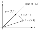
Exact Euclidean coordinates: $p^Tr=0$. The residual is not a vertical error to the diagonal line.

D. Least squares is projection onto the column space#

For $p=Ax$ to be the projection of $b$, its residual must satisfy $A^T(b-Ax)=0$. Thus the normal equations are

When $A$ has independent columns, $A^TA$ is invertible: for nonzero $z$, $z^TA^TAz=\|Az\|^2>0$. If columns are dependent, minimizers need not be unique, although the projected vector $Ax$ is unique. Explicitly forming the inverse is not the preferred numerical algorithm. A QR factorization $A=QR$, with orthonormal columns in $Q$ and upper triangular $R$, reduces the problem to $Rx=Q^Tb$. The lab uses modified Gram–Schmidt to illustrate this geometry. More robust libraries use methods such as Householder QR or SVD; the small lab is not a replacement for them. [LA]

Fit a line $y\approx\beta_0+\beta_1t$ to $(t,y)=(0,1),(1,2),(2,2)$. Then

Subtract the first normal equation from the second to get $2\beta_1=1$, hence $\beta_1=1/2$ and $\beta_0=7/6$. Predictions are $7/6,5/3,13/6$ and residuals $-1/6,1/3,-1/6$. Their sum is zero, and their dot product with $(0,1,2)$ is zero. Those two checks verify perpendicularity to both design columns. The line minimizes squared vertical response residuals at fixed $t$, not arbitrary geometric distances in the $(t,y)$ plane.

E. Eigenvectors identify directions preserved by a square map#

An eigenvector is a nonzero vector $v$ satisfying $Av=\lambda v$. The scalar $\lambda$ is its eigenvalue. The zero vector is excluded because it satisfies the equation for every $\lambda$ and would identify no direction. Eigenvalues solve $\det(A-\lambda I)=0$, but deriving the characteristic polynomial by hand is not the default stable algorithm for a large matrix.

For $A=\begin{pmatrix}2&1\\1&2\end{pmatrix}$, vectors $(1,1)$ and $(1,-1)$ have eigenvalues 3 and 1. Normalize them to form an orthogonal matrix $Q$; then $A=Q\operatorname{diag}(3,1)Q^T$. In those coordinates, repeated application simply multiplies the two components by powers of 3 and 1. This explains why one direction dominates long-term growth. Symmetric real matrices admit an orthonormal eigenbasis; a general matrix may not, may have complex eigenvalues, or may lack enough independent eigenvectors.

A real symmetric matrix is positive definite when $x^TAx>0$ for every nonzero real $x$. Its eigenvalues are then positive, and a quadratic energy $\frac12x^TAx$ curves upward in every direction. Positive diagonal entries alone do not establish this property. For a symmetric $2\times2$ matrix, the first leading diagonal entry and determinant being positive are sufficient. In higher dimensions, use an appropriate criterion or factorization, not a guessed extension of a two-dimensional rule.

F. Singular values separate rotations from stretching#

For any real $m\times n$ matrix, an SVD has the form $A=U\Sigma V^T$, with orthogonal square $U,V$ and rectangular nonnegative diagonal $\Sigma$. Read this right to left: change input coordinates, stretch or erase principal directions, then change output coordinates. The nonzero singular values are square roots of the positive eigenvalues of $A^TA$. They apply to rectangular maps and describe directional gains even when eigenvectors of $A$ itself are not appropriate.

For $A=\begin{pmatrix}1&1\\0&0\end{pmatrix}$, the input direction $(1,1)/\sqrt2$ is stretched by $\sqrt2$ to output direction $(1,0)$, while $(1,-1)/\sqrt2$ is erased. The rank is one. Keeping the largest singular directions gives a low-rank approximation; the truncated SVD has an optimality theorem for specified matrix norms, but it does not automatically preserve the features that a human application considers important. Numerical rank also requires a tolerance relative to scale and measurement uncertainty.

G. Independent practice#

F foundation C standard course work T transfer S optional stretch L runnable lab or project. Attempt the complete set before opening its solutions.

H. Complete solutions: A02#

Compare the first step where your work differs. A corrected answer is not yet an independent success.

Open every solution

"""A02.05: modified Gram-Schmidt QR for a small full-column-rank matrix."""
import math

def least_squares(a: list[list[float]], b: list[float],
                  tolerance: float = 1e-12) -> list[float]:
    m = len(a)
    n = len(a[0]) if m else 0
    if not n or m < n or len(b) != m or any(len(row) != n for row in a):
        raise ValueError("a must be rectangular, m >= n; b must have m entries")
    if tolerance <= 0 or not math.isfinite(tolerance):
        raise ValueError("positive finite tolerance required")
    if any(not math.isfinite(v) for row in a for v in row) or any(
            not math.isfinite(v) for v in b):
        raise ValueError("finite data required")
    q: list[list[float]] = []
    r = [[0.0] * n for _ in range(n)]
    for j in range(n):
        v = [row[j] for row in a]
        for i in range(j):
            r[i][j] = math.fsum(q[i][k] * v[k] for k in range(m))
            v = [v[k] - r[i][j] * q[i][k] for k in range(m)]
        r[j][j] = math.sqrt(math.fsum(x * x for x in v))
        if r[j][j] <= tolerance:
            raise ValueError("numerically dependent columns at chosen tolerance")
        q.append([x / r[j][j] for x in v])
    y = [math.fsum(col[k] * b[k] for k in range(m)) for col in q]
    x = [0.0] * n
    for i in range(n - 1, -1, -1):
        x[i] = (y[i] - math.fsum(r[i][j] * x[j]
                                 for j in range(i + 1, n))) / r[i][i]
    return x

if __name__ == "__main__":
    print(least_squares([[1., 0.], [1., 1.], [1., 2.]], [1., 2., 2.]))

I. Retention and readiness#

Retrieve rank–nullity and the geometric meaning of a matrix column. Advance when you can derive a projection from perpendicularity, explain what least squares minimizes, and distinguish eigenvalues from singular values. Continue with numerical linear algebra and larger QR/SVD experiments before treating this introduction as advanced competence.