Module 07: Continuity, existence, and precise limit reasoning

8 exercises, each with a complete solution. 1 figure.

On this page

A. Prerequisites and observable goals
B. The central idea: connect nearby behavior to the actual value
C. Definitions and theorem conditions
D. Why epsilon–delta is more than symbolism
E. A decision procedure
F. Worked examples
G. Independent practice
H. Complete solutions: Module 07
I. Retention and readiness

A. Prerequisites and observable goals#

Before

One-sided limits, absolute value, and solving simple inequalities.

After

Test continuity, apply the Intermediate Value Theorem with its assumptions, and construct simple epsilon–delta proofs.

B. The central idea: connect nearby behavior to the actual value#

A limit describes nearby outputs. Continuity adds the requirement that the nearby behavior agrees with the output at the point. A continuous graph may be very steep and need not be smooth; continuity concerns output closeness, not existence of a slope.

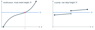
The Intermediate Value Theorem (IVT) turns continuity into an existence guarantee. A continuous function cannot go from below a height to above it without attaining that height somewhere in between. The theorem does not tell us an exact crossing input or guarantee only one crossing.

The Intermediate Value Theorem needs continuity. Left: a continuous curve that starts below the height

N

and ends above it must meet that height at some input

c

. Right: with a jump, the function passes from below

N

to above it without ever taking the value

N

C. Definitions and theorem conditions#

A function $f$ is continuous at $a$ when $f(a)$ is defined and

\lim_{x\to a}f(x)=f(a).

At an endpoint of its domain, use the appropriate relative, one-sided version. Continuity on $[a,b]$ means continuity inside the interval with right continuity at $a$ and left continuity at $b$ .

A removable discontinuity has a finite common limit but a missing or mismatched point value. A jump has different finite one-sided limits. Infinite behavior is another way continuity can fail. Polynomials are continuous everywhere; quotients of continuous functions are continuous where their denominators are nonzero.

The precise finite limit definition is

\forall\varepsilon>0\ \exists\delta>0:\qquad 0<|x-a|<\delta\Longrightarrow |f(x)-L|<\varepsilon

for domain inputs $x$ . Read $\varepsilon$ as an output tolerance and $\delta$ as an input tolerance. The quantifier order matters: after the output tolerance is chosen, we must supply an input tolerance that works for every sufficiently close domain input, not just a few samples. The input $a$ must be an accumulation point of the domain for this usual limit discussion. Definitions and IVT checked against [O1L].

D. Why epsilon–delta is more than symbolism#

To prove $\lim_{x\to2}(3x-1)=5$ , examine the output error:

|(3x-1)-5|=3|x-2|.

To force this below a requested $\varepsilon$ , choose $\delta=\varepsilon/3$ . Then $0<|x-2|<\delta$ implies the desired output error is below $3\delta=\varepsilon$ . We did not guess a tiny numerical input change; we produced a rule valid for every positive tolerance.

For a nonlinear example, $|x^2-4|=|x-2||x+2|$ . We control $|x-2|$ directly but need to bound $|x+2|$ . First insist $|x-2|<1$ , which implies $1<x<3$ and $|x+2|<5$ . Now

|x^2-4|<5|x-2|.

Choose $\delta=\min(1,\varepsilon/5)$ . One part keeps $x$ local; the other controls the output error. This local-bound idea returns in multivariable limits.

E. A decision procedure#

For continuity, check point value, two-sided limit, and equality in that order. For a piecewise function, use branch formulas to compare one-sided limits at the joining input. For IVT, explicitly state continuity on the entire closed interval and show the target lies between the endpoint outputs. Do not conclude uniqueness without another argument, such as strict monotonicity. For an epsilon–delta proof, first work backward from $|f(x)-L|<\varepsilon$ to find a candidate $\delta$ ; then write a forward proof that starts with that choice and establishes the implication.

F. Worked examples#

Joining two branches. Let $f(x)=x^2+k$ for $x<1$ and $f(x)=3x$ for $x\ge1$ . The left limit is $1+k$ , the right limit and point value are both $3$ . Continuity at $1$ requires $1+k=3$ , hence $k=2$ . This solves a matching problem; no derivative is needed.

Existence without an explicit formula. Let $F(x)=x^3+x-1$ . It is a polynomial, hence continuous on $[0,1]$ . Since $F(0)=-1$ and $F(1)=1$ , the IVT guarantees a zero in $(0,1)$ . Finding that zero’s decimal digits is a separate numerical task.

Why a sign change alone is insufficient. The function $1/x$ changes from negative at $-1$ to positive at $1$ , yet it never equals zero. It is not continuous on $[-1,1]$ because it is undefined at $0$ . The missing hypothesis explains the failure; the IVT itself remains valid.

G. Independent practice#

F foundation C standard course work T transfer S optional stretch L runnable lab or project. Attempt the complete set before opening its solutions.

M07.01FSolution

Let $f(x)=(x^2-1)/(x-1)$ for $x\ne1$ , with $f(1)=8$ . Is it continuous at $1$ ? Which new value would make it continuous?

M07.02CSolution

Choose $k$ so that $f(x)=2x+k$ for $x<2$ and $f(x)=x^2-1$ for $x\ge2$ is continuous at $2$ .

M07.03CSolution

Use the IVT to prove that $x^3-2x-2=0$ has a solution in $(1,2)$ . Does this application prove uniqueness?

M07.04TSolution

Explain why endpoint values $f(-1)=-1$ and $f(1)=1$ alone do not guarantee a zero. Give a concrete function counterexample.

M07.05CSolution

Prove $\lim_{x\to1}(4x+2)=6$ using an explicit $\delta$ for every $\varepsilon>0$ .

M07.06SSolution

Prove $\lim_{x\to3}x^2=9$ using $\delta=\min(1,\varepsilon/7)$ . Explain the number $7$ .

M07.07TSolution

Is $|x|$ continuous at $0$ ? Explain without assuming that it has a tangent slope there.

M07.08SSolution

A continuous function on $[0,1]$ satisfies $f(0)=1$ and $f(1)=0$ . Prove that $f(c)=c$ for some $c\in(0,1)$ .

Optional small hints

For M07.06, factor $x^2-9$ and bound $|x+3|$ near $3$ . For M07.08, study the sign of $f(x)-x$ .

H. Complete solutions: Module 07#

Compare the first step where your work differs. A corrected answer is not yet an independent success.

M07.01Show solution

Repair a removable discontinuity

For $x\ne1$ , factoring gives $(x^2-1)/(x-1)=x+1$ . Its limit at $1$ is $2$ , but the assigned value is $8$ . Since they disagree, the function is not continuous. Defining $\boxed{f(1)=2}$ would restore continuity without changing any other input.

Back to M07.01

M07.02Show solution

Match both branches to the actual value

The left limit is $2(2)+k=4+k$ . The right branch is a polynomial and includes $2$ , so both the right limit and $f(2)$ equal $2^2-1=3$ . Set $4+k=3$ , giving $\boxed{k=-1}$ . With this value, the one-sided limits and point value all agree.

Back to M07.02

M07.03Show solution

A justified existence claim

Let $F(x)=x^3-2x-2$ . It is continuous on $[1,2]$ because it is polynomial. Evaluate $F(1)=-3$ and $F(2)=2$ . The target $0$ lies strictly between these values, so IVT gives some $c\in(1,2)$ with $F(c)=0$ . This application proves at least one root, not exactly one; uniqueness would require additional reasoning.

Back to M07.03

M07.04Show solution

The missing continuity hypothesis

Define $f(x)=-1$ for $x<0$ and $f(x)=1$ for $x\ge0$ . It has the stated endpoint values but never takes value zero. The jump at $0$ violates continuity on the interval. Endpoint arithmetic alone therefore cannot replace the IVT’s assumption.

Back to M07.04

M07.05Show solution

A tolerance that works for every nearby input

Given any $\varepsilon>0$ , choose $\delta=\varepsilon/4>0$ . If $0<|x-1|<\delta$ , then

|(4x+2)-6|=4|x-1|<4\delta=\varepsilon.

This establishes the required implication for every allowed nearby input, so the limit is $6$ . The choice of $\delta$ depends on the requested output accuracy.

Back to M07.05

M07.06Show solution

Bound the uncontrolled factor locally

Let $\varepsilon>0$ and choose $\delta=\min(1,\varepsilon/7)$ . If $0<|x-3|<\delta$ , then $2<x<4$ , hence $5<x+3<7$ and $|x+3|<7$ . Consequently

|x^2-9|=|x-3||x+3|<7|x-3|<7\delta\le\varepsilon.

The $7$ is an upper bound for the other factor while $x$ stays within $1$ of $3$ . It is convenient, not uniquely required.

Back to M07.06

M07.07Show solution

Continuity does not require a derivative

The value is $|0|=0$ . Also, as $x\to0$ , $||x|-0|=|x|\to0$ , so the limit equals the point value. Thus $|x|$ is continuous at $0$ . This says nothing yet about its tangent slope; Module 08 will show that its left and right slope limits disagree.

Back to M07.07

M07.08Show solution

Turn a crossing question into a zero question

Set $g(x)=f(x)-x$ . Both $f$ and $x$ are continuous on $[0,1]$ , so $g$ is too. Its endpoint values are $g(0)=1$ and $g(1)=-1$ . By IVT, some $c\in(0,1)$ satisfies $g(c)=0$ , which means $\boxed{f(c)=c}$ . Introducing the difference identifies the correct function to which the theorem applies.

Back to M07.08

I. Retention and readiness#

Mix M06.05 with M07.01 to distinguish a missing common limit from a wrong point value. Recite the IVT assumptions and its limited conclusion. Epsilon–delta proofs are optional depth at first, but their meaning is not: a limit controls all sufficiently close inputs, not only a handpicked table. Revisit the nonlinear proof after the derivative definition feels secure.