C08: Trees, heaps, graphs, and shortest-path reasoning

A. Prerequisites and observable goals#

Level: Degree core.

B. The central question: how should relationships be represented and explored?#

A graph $G=(V,E)$ can be directed or undirected, weighted or unweighted. These are not cosmetic labels. A route allowed from $u$ to $v$ need not be allowed in reverse. An edge weight may represent distance, latency, or cost; summing it along a path requires compatible units and an appropriate objective. A disconnected graph has vertices that cannot be reached from a chosen source. An algorithm should represent that state explicitly instead of assigning a fabricated finite distance.

An adjacency list stores the outgoing neighbors of each vertex and uses $O(|V|+|E|)$ space in the standard representation. An adjacency matrix uses $O(|V|^2)$ space but gives direct edge-presence lookup. Sparse graphs often favor lists; dense or matrix-oriented computations can favor matrices. Multiple edges, self-loops, and vertex identifiers need explicit policies. The lab accepts a declared vertex mapping with finite nonnegative weighted edges and rejects references to missing vertices.

C. A tree is not necessarily a balanced search structure#

A binary search tree stores keys so that keys in a left subtree precede the node’s key and keys in the right subtree follow it, under a declared duplicate policy. Search follows a root-to-leaf path, costing $O(h)$ for height $h$. Inserting sorted keys into a naive tree can produce height $n-1$, so “tree lookup is logarithmic” is false without a balance guarantee or suitable distribution assumption.

Balanced-tree families maintain additional invariants. An AVL tree bounds the height difference of child subtrees and uses local rotations after updates. A rotation changes parent-child links while preserving in-order key order. Red-black trees maintain coloring and black-height constraints that bound height logarithmically. This module introduces the balancing idea, not a complete verified implementation of either family. Implementing rotations, deletion, and iterator invalidation safely is a substantial continuation exercise, not a one-line extension.

A binary min-heap instead requires every parent key to be no greater than its children. It does not order all left-subtree keys before all right-subtree keys. In a zero-based array, children of index $i$ are $2i+1$ and $2i+2$ when present; the parent of $i>0$ is $\lfloor(i-1)/2\rfloor$. Insertion appends then repairs upward; extracting the minimum moves the last element to the root then repairs downward. Both repairs follow one path of logarithmic height. Bottom-up heap construction is $O(n)$ because most nodes are close to leaves; summing work by height gives a convergent bound proportional to $n\sum_{h\ge0}h/2^h$.

D. BFS and DFS answer different questions#

Breadth-first search uses a FIFO queue. Mark a vertex discovered when enqueuing it, set its distance one more than the current vertex’s, and record its predecessor. The queue processes vertices in nondecreasing edge-count distance, so first discovery gives a shortest path in an unweighted or uniformly weighted graph. It does not minimize arbitrary unequal weights. With adjacency lists, every vertex and edge is processed a bounded number of times, giving $O(|V|+|E|)$ work.

Depth-first search uses a stack, explicit or recursive, to pursue one branch before returning. It supports reachability, connected components in undirected graphs, cycle analysis, and topological ordering for directed acyclic graphs. In a directed graph, distinguishing undiscovered, active, and finished vertices detects a back edge to the active path. A topological order exists only for a DAG. Reversing a valid DFS finishing order gives one such order after cycle checks; doing so blindly on a cyclic graph does not remove the cycle.

E. Dijkstra’s algorithm needs nonnegative weights#

Initialize the source distance to zero and others to infinity. Repeatedly remove the smallest tentative distance from a priority queue. Relax an outgoing edge $(u,v)$ by comparing the current best $d(v)$ with $d(u)+w(u,v)$. A smaller candidate replaces the distance and predecessor and enters the heap. The lab uses lazy deletion: old heap entries remain but are ignored when their stored distance no longer equals the current best.

The correctness argument is a frontier argument. Suppose the smallest unsettled tentative vertex $u$ had a truly shorter path. Follow that path until its first unsettled vertex $y$, whose predecessor was already settled. Relaxation from that predecessor would have made $d(y)$ no greater than the corresponding path prefix. With nonnegative remaining edges, that prefix cannot exceed the supposedly shorter path to $u$, contradicting $u$ being selected with the smallest tentative distance. Negative edges break this comparison. Bellman–Ford is a continuation for negative edges and detection of reachable negative cycles.

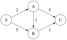
Directed graph with abstract nonnegative cost units. The best S-to-C path costs $2+1+1=4$, not 7.

For this graph, S first proposes A at 2 and B at 5. A improves B to 3 and proposes C at 7. B improves C to 4. Stale entries B at 5 and C at 7 do not invalidate the result; they must be skipped when removed. Predecessors reconstruct S–A–B–C.

For the lazy-heap implementation, at most one successful decrease is generated per examined edge. A safe bound is $O(|V|+|E|+(|E|+1)\log(|E|+2))$ work and $O(|V|+|E|)$ storage. For simple graphs this is commonly simplified to the familiar logarithm-in-vertices bound. State the implementation and graph model instead of silently assuming a decrease-key heap. Floating-point weights also introduce rounding in nearly tied path sums; finite-value checks do not establish exact real-arithmetic ranking at arbitrary precision.

F. Spanning trees solve a different optimization problem#

A shortest-path tree minimizes source-to-vertex path distances. A minimum spanning tree minimizes the sum of selected edge weights needed to connect all vertices of a connected undirected graph. These objectives differ. Kruskal’s algorithm sorts edges by weight and accepts an edge when it connects two previously disconnected components. The cut property justifies accepting a lightest edge across an appropriate component cut: an optimal spanning tree can exchange another crossing edge for it without increasing total weight.

A disjoint-set union structure tracks components. Each element points toward a representative; union joins roots, and path compression shortens future searches. Union by rank or size avoids long naive chains. The well-known near-constant amortized bound with both techniques is not a worst-case constant guarantee for each operation. With disconnected input, Kruskal produces a minimum spanning forest. Negative edge weights are allowed in this problem; Dijkstra’s nonnegativity restriction must not be transferred blindly to every graph algorithm.

G. Independent practice#

F foundation C standard course work T transfer S optional stretch L runnable lab or project. Attempt the complete set before opening its solutions.

H. Complete solutions: C08#

Compare the first step where your work differs. A corrected answer is not yet an independent success.

Open every solution

"""C08.05: Dijkstra; vertices are strings and weights finite/nonnegative."""
import heapq
import math

def shortest_paths(graph: dict[str, list[tuple[str, float]]],
                   start: str) -> tuple[dict[str, float], dict[str, str]]:
    if start not in graph:
        raise ValueError("missing start vertex")
    if any(not isinstance(u, str) for u in graph):
        raise TypeError("string vertices required")
    for edges in graph.values():
        for v, w in edges:
            if v not in graph or not math.isfinite(w) or w < 0:
                raise ValueError("invalid endpoint or weight")
    dist = {u: math.inf for u in graph}
    prev: dict[str, str] = {}
    dist[start] = 0.0
    heap = [(0.0, start)]
    while heap:
        d, u = heapq.heappop(heap)
        if d != dist[u]:
            continue
        for v, w in graph[u]:
            new = d + w
            if not math.isfinite(new):
                raise OverflowError("path cost overflow")
            if new < dist[v]:
                dist[v], prev[v] = new, u
                heapq.heappush(heap, (new, v))
    return dist, prev

if __name__ == "__main__":
    g = {"a": [("b", 4), ("c", 1)], "b": [], "c": [("b", 2)]}
    print(shortest_paths(g, "a")[0])

I. Retention and readiness#

Retrieve queue versus stack behavior, heap invariants, and the difference between a path and a spanning tree. Advance when you can trace a new graph without running it, state each algorithm’s hypotheses, and explain why a tempting alternative optimizes the wrong quantity.