G03: Algorithm design, certificates, and honest complexity

Prerequisites and observable goals#

The central question: how can a result carry evidence?#

Some problems have compact certificates. A path proves reachability, but not necessarily shortest distance. A feasible flow and a cut of the same value jointly prove optimality. A dynamic program can provide a reconstruction of its choices. Design the certificate while designing the algorithm: it creates an independent way to challenge a plausible-looking result.

Start with the problem’s quantifiers and constraints. “Choose a cheapest subset” is not enough. What does the subset need to cover? Are costs nonnegative? Can one item be used multiple times? Are decisions divisible? A small change may turn greedy selection from correct into wrong, or require a different state in a dynamic program.

A derived dynamic program: nonadjacent tasks#

Suppose tasks lie in a chain, each has value $v_i\ge0$, and adjacent tasks cannot both be selected. Let $D[i]$ be the greatest value achievable using only tasks $1$ through $i$. A solution either excludes task $i$, leaving value at most $D[i-1]$, or includes it, excluding $i-1$ and leaving at most $v_i+D[i-2]$. These alternatives are exhaustive, so

Induction proves optimality: assume the smaller prefixes are solved optimally; every feasible prefix solution belongs to one of the two cases and cannot beat the larger expression; combining the appropriate optimal smaller solution achieves that expression. The recurrence is not a slogan about “optimal substructure”; it is a proof by a last-decision partition.

For values $(4,7,5,6)$, the table is $D[0..4]=(0,4,7,9,13)$. Reconstruction starts at $i=4$: $13=6+D[2]$, so take 4 and continue at 2. Take 2 for a total $7+6=13$. Greedily taking the largest remaining individual value happens to succeed here but fails on $(6,10,6)$: picking the middle 10 loses to both endpoints totaling 12.

The table uses $O(n)$ arithmetic comparisons and additions. Value-only computation can retain two prior entries, using $O(1)$ auxiliary slots. Reconstructing choices then needs stored decisions or recomputation. Large integer bit costs also matter when values are not bounded machine words.

Flow, residual capacity, and reversible decisions#

A directed network has source $s$, sink $t$, nonnegative capacities $c(u,v)$, and conservation at internal vertices. A conventional feasible flow has nonnegative edge quantities bounded by capacities. For implementation with possible edges in both directions, it is convenient to track a net antisymmetric flow $f(u,v)=-f(v,u)$ with $f(u,v)\le c(u,v)$. Residual capacity is

Increasing net flow by $\delta$ on $(u,v)$ decreases $r(u,v)$ and increases $r(v,u)$. The reverse residual edge is permission to undo a prior decision, not a new physical network link. A residual algorithm that omits reverse updates can get stuck below the optimum.

Consider four vertices $(s,a,b,t)$ with capacities $s\to a=3$, $s\to b=2$, $a\to b=1$, $a\to t=2$, and $b\to t=3$. Send two units along $s,a,t$, two along $s,b,t$, then one along $s,a,b,t$. The total is five. The cut separating $s$ alone has outgoing capacity $3+2=5$, so no flow can exceed five. The constructed flow and cut certify one another.

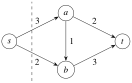
Labels are capacities, not measured bandwidth. The dashed cut crosses exactly the source’s two outgoing arcs. Flow conservation makes internal movement cancel when computing net flow through a cut.

Why the terminal residual cut proves optimality#

For any cut $S$ containing $s$ but not $t$, the total flow value equals net flow leaving $S$: contributions between vertices inside $S$ cancel in pairs, and internal vertices conserve flow. Net outgoing flow cannot exceed the sum of capacities from $S$ to its complement. Thus every cut is an upper bound.

When no residual path from $s$ to $t$ remains, let $S$ be all vertices reachable from $s$ by positive residual arcs. Every arc from $S$ outward has zero residual, otherwise its endpoint would be reachable. Therefore net flow on each such arc equals its capacity. Summing gives a flow equal to that cut’s capacity, meeting the upper bound. Hence the flow is maximum and the cut minimum. This argument is a proof of the certificate condition, not merely empirical agreement. The lab’s integer capacities also guarantee each successful augmentation makes positive integral progress. [G-FLOW]

Complexity belongs to a representation#

Edmonds–Karp chooses a shortest-in-edge-count residual path by BFS. The standard augmentation argument bounds successful augmentations by $O(VE)$: residual shortest distances do not decrease, and a particular directed edge can become critical only $O(V)$ times as its relevant distance increases. With adjacency lists, a BFS is $O(V+E)$, giving the familiar $O(VE^2)$ bound after restricting to the relevant graph. This is not a generic bound for arbitrary path selection.

Our educational implementation scans all $V$ entries of a residual-matrix row for each visited vertex. One BFS costs $O(V^2)$ even on sparse graphs. Combining the augmentation bound with these scans yields $O(V^3E)$ as a conservative operation bound, plus the final BFS; for $E=0$ the initial $O(V^2)$ work still exists. State the bound as $O(V^2+V^3E)$. Storage is $O(V^2)$. Copying a sparse matrix and calling it an adjacency list would not change the executed work.

Amortized, expected, and approximate are different#

For a dynamic array doubling capacity on a full insertion, most insertions are cheap and a few copy many elements. At capacity $C$ and size $n$ after at least the first insertion, use potential $\Phi=2n-C\ge0$ for the usual doubling regime. An ordinary insertion costs one and increases potential by two, giving amortized cost three. A full insertion from $n=C$ costs $C+1$, changes capacity to $2C$, and changes potential from $C$ to 2; amortized cost is $(C+1)+(2-C)=3$. Initial allocation is handled separately. This pays for an expensive deterministic event by accounting across a sequence; it is not a probability claim.

Expected hash-table lookup depends on a randomness/input model. A 2-approximation bound compares a feasible result with an unknown optimum for every permitted instance; it does not mean “wrong half the time.” NP-completeness concerns polynomial reductions and verification, not a blanket prohibition on useful exact solutions for bounded or structured instances. When an exact method is too costly, make the tradeoff explicit: approximate objective, restricted input class, probabilistic failure, or a resource cutoff with an incomplete answer.

Independent practice#

F foundation C standard course work T transfer S optional stretch L runnable lab or project. Attempt the complete set before opening its solutions.

Smallest useful hints#

For .01, partition on whether the last task is chosen. For .03, the path may use a reverse residual edge. For .06, copying the matrix avoids mutating a caller’s capacity data; do not mistake residual capacity for original capacity when evaluating the certificate.

Complete solutions: G03#

Compare the first step where your work differs. A corrected answer is not yet an independent success.

Open every solution

"""G03: Edmonds-Karp with a residual matrix and a min-cut certificate."""
from collections import deque


def max_flow(capacity, source, sink):
    n = len(capacity)
    if not 2 <= n <= 64 or any(len(row) != n for row in capacity):
        raise ValueError("square capacity matrix with 2..64 vertices required")
    if any(type(c) is not int or c < 0 for row in capacity for c in row):
        raise ValueError("nonnegative integer capacities required")
    if (type(source) is not int or type(sink) is not int
            or not 0 <= source < n or not 0 <= sink < n or source == sink):
        raise ValueError("distinct valid source and sink required")
    if any(capacity[i][i] != 0 for i in range(n)):
        raise ValueError("self-loop capacities must be zero")
    residual = [list(row) for row in capacity]
    value = 0
    while True:
        parent = [-1] * n
        parent[source] = source
        todo = deque([source])
        while todo and parent[sink] == -1:
            u = todo.popleft()
            for v in range(n):
                if residual[u][v] > 0 and parent[v] == -1:
                    parent[v] = u
                    todo.append(v)
        if parent[sink] == -1:
            reachable = {i for i, p in enumerate(parent) if p != -1}
            return value, reachable, residual
        delta = None
        v = sink
        while v != source:
            u = parent[v]
            delta = residual[u][v] if delta is None else min(delta, residual[u][v])
            v = u
        v = sink
        while v != source:
            u = parent[v]
            residual[u][v] -= delta
            residual[v][u] += delta
            v = u
        value += delta


def cut_capacity(capacity, reachable):
    return sum(c for u, row in enumerate(capacity) for v, c in enumerate(row)
               if u in reachable and v not in reachable)


if __name__ == "__main__":
    c = [[0, 3, 2, 0], [0, 0, 1, 2], [0, 0, 0, 3], [0, 0, 0, 0]]
    value, side, _ = max_flow(c, 0, 3)
    print(value, sorted(side), cut_capacity(c, side))

Readiness and continuation#

Explain the reverse edge without using the phrase “because the algorithm says so.” Show why no residual path gives a cut certificate. Then change the representation and recalculate cost. Further work can add min-cost flow, approximation proofs, randomized concentration bounds, and fixed-parameter methods; none is claimed implemented by this lab. Use the original maximum-flow chapter for a fuller proof of the shortest-augmenting-path complexity bound. [G-FLOW]