A03: Probability, random variables, and simulation
On this page
- A. Prerequisites and observable goals
- B. The central question: what can be known before an uncertain outcome occurs?
- C. Conditioning changes the population under consideration
- D. A rare-event calculation with actual counts
- E. Random variables turn outcomes into quantities
- F. Select distributions by their generating assumptions
- G. Independent practice
- H. Complete solutions: A03
- I. Retention and readiness
A. Prerequisites and observable goals#
Fractions, sets, finite sums, and basic function notation. Integrals from Modules 16–17 support continuous distributions.
Compute conditional probabilities without reversing them, distinguish independence from exclusivity, derive expectations and variances, and choose a probability model from assumptions rather than appearance.
Level: Degree core.
B. The central question: what can be known before an uncertain outcome occurs?#
A probability model consists of a sample space of possible outcomes, events that are subsets of that space, and a probability assignment. Probability is not a synonym for a personal feeling of confidence: calculations are conditional on the specified model. A fair six-sided die has six equally probable elementary outcomes; a production server’s next latency need not have equally likely values, independence across requests, or an unchanging distribution.
For an event , , and the whole sample space has probability one. For disjoint events, probabilities add. General addition requires subtracting overlap:
A count divided by a total gives a probability only when the counted elementary outcomes are equally probable. Ordered outcomes and unordered selections are different sample spaces. For example, selecting two distinct items from five gives ordered pairs but unordered pairs. Each unordered pair corresponds to two orders. Counting foundations are developed further in C05; probability uses those counts only under a justified sampling rule.
C. Conditioning changes the population under consideration#
For ,
The vertical bar means “within outcomes where occurred.” It does not reverse the direction of a causal relationship. Events are independent when . For positive , this is equivalent to . Disjoint events with positive probabilities are not independent: learning that one occurred rules out the other.
Bayes’ theorem rearranges the same joint probability:
If and partition the possibilities, then . This denominator accounts for every route to observing , including false alarms. A system’s sensitivity is not the probability that a flagged case is genuine.
D. A rare-event calculation with actual counts#
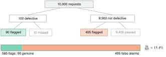
Suppose 1% of requests are genuinely defective, a detector flags 90% of defective requests, and it falsely flags 5% of nondefective requests. In a model population of 10,000 requests, expect 100 defective requests, 90 true flags, and false flags. Among 585 total flags, only 90 are genuine:
This does not make the detector useless. It shows why its operating threshold, base rate, and cost of false positives matter. A different population with a higher defect rate changes the posterior even when sensitivity and false-positive rate remain the same. The numerical result is conditional on those assumptions; it is not an empirical claim about a real system.
E. Random variables turn outcomes into quantities#
A random variable is a function from outcomes to numbers. For a discrete variable, its mass function is and
Expectation is a probability-weighted average, not necessarily a possible observed value. Variance has squared units; standard deviation has the original units. For a continuous density , probabilities are integrals over intervals, and when the expectation is well-defined. A density can exceed one over a short interval; its integral over the whole domain must equal one. A continuous variable’s probability at a single point is zero even when that point lies in its support.
Linearity of expectation does not require independence: when the expectations exist. Variance does require attention to dependence:
Independence implies zero covariance when the relevant moments exist, but zero covariance does not generally imply independence. Shared server congestion can make two request latencies positively dependent, increasing the variability of their sum.
An indicator equals 1 if occurs and 0 otherwise. Then . A binomial count for independent, identical Bernoulli trials has mean and variance . The derivation exposes exactly where identical probabilities and independence enter; it is more useful than remembering a distribution name.
F. Select distributions by their generating assumptions#
| Model | Interpretation and conditions | Mean; variance |
|---|---|---|
| Bernoulli | One event, coded 0 or 1 | ; |
| Binomial | Count in independent identical trials | ; |
| Geometric | Number of independent trials through first success; starts at 1 | ; |
| Poisson | Count in a model interval with specified intensity and suitable independent-increment assumptions | ; |
| Uniform | Constant density on a finite interval, | ; |
| Exponential | Waiting time in a constant-rate memoryless model, | ; |
| Normal | Symmetric continuous model; often an approximation, not a law of all noise | ; |
A normal model permits negative values, so applying it to latency requires a justified approximation over the relevant range. An exponential model’s memorylessness is a substantive assumption, not a property of every wait. Fit and validate a model against the mechanism and observations; do not choose it only because its formula is convenient. [PROB]
For a synthetic latency equal to 10 ms with probability 0.95 and 110 ms with probability 0.05, ms. But 15 ms is never observed. Its variance is . The average hides the 110 ms tail. A capacity or responsiveness requirement needs appropriate tail behavior as well as a mean.
G. Independent practice#
F foundation C standard course work T transfer S optional stretch L runnable lab or project. Attempt the complete set before opening its solutions.
A uniformly selected unordered pair comes from five distinct items. What is the probability that a particular item is included? Derive the result by counting, not by assuming the two selections are independent.
Recompute the detector posterior when the defect rate is 10%, sensitivity remains 90%, and false-positive rate remains 5%. Explain why the posterior changes.
For the two-point latency model above, compute the expectation and variance of the sum of two independent latencies. Then explain which calculation survives if independence is removed and which additional quantity the variance needs.
Let be uniform on and . Show that their covariance is zero but they are not independent. Explain why “uncorrelated” is a weaker statement.
Implement the seeded binomial experiment in probability_lab.py. Generate independent pseudo-random Bernoulli trials, group them into counts, and compare the sample mean and variance with and . Validate , , and the number of repetitions. Record the seed and explain why a close sample result is not a proof of the formulas.
Optional small hints
A03.01: count pairs containing the chosen item. A03.04: compute . A03.05: derive the expected quantities analytically before generating any samples.
H. Complete solutions: A03#
Compare the first step where your work differs. A corrected answer is not yet an independent success.
A03.01Show solution
Count the relevant sample space
There are equally likely unordered pairs. Exactly four include the specified item, one for each possible partner. The probability is . The selections without replacement are dependent, but the combinatorial model already accounts for that. Summing five inclusion indicators gives exactly two for every pair; symmetry provides the independent check .
Back to A03.01A03.02Show solution
The base rate changes the mixture
The joint probability of a genuine flag is . The false-flag probability is . Thus the posterior is . The detector’s conditional operating rates are unchanged, but a greater fraction of requests belongs to the defective population. The observed flags therefore contain a larger fraction of genuine cases. Conditioning cannot ignore population composition.
Back to A03.02A03.03Show solution
Means add more generally than variances
The expected sum is ms. Under independence, the variance is . Without independence the expectation remains 30 ms because linearity does not require it. The variance becomes in squared milliseconds. A shared slow state could make the covariance positive; negative dependence could reduce it. Do not add standard deviations as though they were variances.
Back to A03.03A03.04Show solution
Dependence can be nonlinear
, , and . Hence covariance is . Yet , whereas . Therefore and are dependent. Covariance detects a particular linear association, not every functional dependence. Here is completely determined by .
Back to A03.04A03.05Show solution
Reference experiment
"""A03.05: seeded binomial experiment with analytic comparison."""
import random
import statistics

def binomial_experiment(n: int = 10, p: float = 0.3,
                        trials: int = 10000, seed: int = 41) -> dict:
    if type(n) is not int or n < 0 or not 0 <= p <= 1:
        raise ValueError("invalid binomial parameters")
    if type(trials) is not int or trials < 2:
        raise ValueError("at least two trials required")
    rng = random.Random(seed)
    data = [sum(rng.random() < p for _ in range(n)) for _ in range(trials)]
    return {"sample_mean": statistics.mean(data),
            "sample_variance": statistics.variance(data),
            "theory_mean": n * p, "theory_variance": n * p * (1 - p),
            "trials": trials, "seed": seed}

if __name__ == "__main__":
    print(binomial_experiment())
Each uniform pseudo-random draw is compared with to form an indicator. The sum of such indicators is one binomial-model observation. The sample variance uses a denominator of trials minus one, which estimates population variance under the independent sampling model. For the default , the analytical targets are 3 and 2.1. The stored seed makes this particular algorithm and environment reproducible, not cryptographically unpredictable. Sampling variation remains even with correct code. A seeded experiment is a check on the implementation and a lesson in variability, while the indicator derivation establishes the theoretical moments under the model assumptions.
Back to A03.05I. Retention and readiness#
Retrieve fractions, inclusion–exclusion, and the difference between a density and an area. Advance when you can name the conditioning population, reject independence when evidence does not support it, and explain a mean that is never itself observed.