Module 17: The Fundamental Theorem, substitution, and area

A. Prerequisites and observable goals#

B. The central idea: accumulation and differentiation undo each other#

Let $A(x)=\int_a^x f(t)\dd t$. The input $x$ moves the upper boundary of an accumulation; $t$ is a dummy variable used inside the integral. Increasing $x$ by a small $h$ adds a thin strip. If the rate is continuous, that strip’s average height approaches $f(x)$, so $A'(x)=f(x)$. This connects the integral’s definition by sums with the practical evaluation of antiderivatives.

C. Two parts of the theorem, and their conditions#

These are convenient sufficient hypotheses for the Fundamental Theorem of Calculus (FTC). An integral of a discontinuous function may still exist, but differentiability of its accumulation needs examination at a discontinuity. [O1FTC]

The chain rule gives

where the relevant continuity and differentiability hold. For two moving bounds, subtract the corresponding lower-bound term. The variable $t$ disappears when the integral has been differentiated.

Substitution is the chain rule reversed. If $u=g(x)$, then the differential shorthand $\dd u=g'(x)\dd x$ records a change in the variable of integration. For definite integrals,

under appropriate continuity and differentiability assumptions. These oriented bounds already account for whether $g$ increases or decreases; this one-dimensional chain-rule substitution does not require $g$ to be globally one-to-one.

Geometric area between continuous graphs is $\int_a^b|f-g|\dd x$. Solve for intersections and determine the upper graph on each subinterval. Integrating “top minus bottom” without checking their order can subtract away real area.

D. Why an accumulation has the original rate#

For small nonzero $h$,

This is the average height over a shrinking interval, with orientation handled by both the integral and $h$. Continuity makes all nearby heights close to $f(x)$, so the quotient tends to $f(x)$. Then $A-F$ has derivative zero and is constant. Evaluating at $a$ gives $A(x)=F(x)-F(a)$, and at $b$ yields the evaluation formula. This argument explains both parts rather than treating bracket notation as the definition of integration.

E. A decision procedure#

First decide whether the problem asks for a derivative of an integral, an integral value, or geometric area. For a derivative, apply FTC and then chain rules for moving bounds. For an integral, simplify algebraically and look for a nested expression whose derivative is also present. In substitution, write $u$, $\dd u$, and either transformed bounds or a clear return to $x$. Never use $x$-bounds on a $u$-antiderivative. For area, draw or compare the graphs before choosing a sign.

F. Worked teaching examples#

A moving endpoint. If $A(x)=\int_1^{x^2}\sqrt{1+t^3}\dd t$ on a neighborhood where the integrand is real and continuous, then $A'(x)=2x\sqrt{1+x^6}$. There is no need to find an elementary antiderivative of the square root. FTC can answer a derivative question even when integration is difficult.

A definite substitution. Evaluate $\int_0^1 2x e^{x^2}\dd x$. Let $u=x^2$, so $\dd u=2x\dd x$, and the bounds become $0,1$. The integral is $\int_0^1e^u\dd u=e-1$. The $2x$ has become part of $\dd u$; it is not an extra factor to retain.

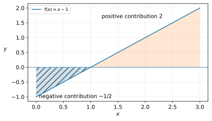
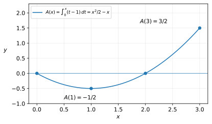
Signed area versus total area. For $f(x)=x-1$ on $[0,3]$, the triangular portion below the axis has area $1/2$ and the portion above has area $2$. Thus the integral is $-1/2+2=3/2$, while geometric area is $1/2+2=5/2$. The accumulation $A(x)=x^2/2-x$ initially decreases, reaches its minimum at $x=1$, and then increases.

Computing bridge: Accumulation and a loop invariant#

A program approximating total distance from sampled velocity might maintain $S_k=\sum_{i=0}^{k-1}v(t_i)\Delta t$. Its loop invariant is that the accumulator equals the contributions processed so far; its physical units are velocity times time. The program can satisfy that invariant perfectly while its approximation is poor because the sampling is coarse or the velocity model is wrong. Calculus separates the exact integral from this finite sum, and J04 separates implementation verification from model validation.

G. Independent practice#

F foundation C standard course work T transfer S optional stretch L runnable lab or project. Attempt the complete set before opening its solutions.

H. Complete solutions: Module 17#

Compare the first step where your work differs. A corrected answer is not yet an independent success.

Open every solution

I. Retention and readiness#

Retrieve M16.04, M10.07, and M12.01. Explain why the dummy variable is not a free variable in the final answer. Advance when you can choose between FTC, substitution, and a sign-based area split without the method being named.