AI01: Autograd from scratch: backpropagation is the chain rule
On this page
- Prerequisites and observable goals
- Warm-up: spaced review (10 minutes, closed book)
- 1. Quick summary
- 2. Deep explanation
- 2.1. The question autograd answers
- 2.2. Partial derivatives: freeze the others
- 2.3. The chain rule on a graph
- 2.4. Used twice? Add the gradients
- 2.5. The order of work: topological sort
- 2.6. Gradient descent: turning gradients into learning
- 2.7. Checking gradients with finite differences
- 2.8. Python for a C++ engineer: exactly what this lab uses
- 2.9. Design trade-offs: why this design, and what breaks at scale
- 2.10. Beginner bugs: a field guide
- 3. The lab: build it yourself
- 3.0. Setup and ground rules
- 3.1. Step 1: a Value that remembers where it came from (worked example)
- 3.2. Step 2: local backward functions (partly filled)
- 3.3. Step 3: backward() for the whole graph (on your own, from the recipe)
- 3.4. Step 4: break it on purpose
- 3.5. Step 5: the remaining operations (on your own)
- 3.6. Step 6: a gradient checker (on your own)
- 3.7. Step 7: neurons, layers, networks (partly filled)
- 3.8. Step 8: teach it XOR (on your own)
- 4. Practice, code reading, and the gate
- 4.1. Practice set
- 4.2. Code-reading drill: micrograd
- 4.3. Mastery gate
- 4.4. Next steps
- 5. Development log entry
- 6. Stretch (optional)
- Hint ladders for the lab
- L1. Step 1: a Value that remembers
- L2. Step 2: local backward functions
- L3. Step 3: backward()
- L4. Step 4: break it on purpose
- L5. Step 5: the remaining operations
- L6. Step 6: the gradient checker
- L7. Step 7: neurons, layers, networks
- L8. Step 8: training
- Complete solutions: AI01
- Retention and readiness
Prerequisites and observable goals#
Calculus I through the chain rule (Modules 08–11): the power rule with negative and fractional exponents, the chain rule, and the derivative of . Python basics (C01–C02) help; section 2.8 covers everything this lab uses, with C++ comparisons.
Compute partial derivatives by freezing the other inputs; backpropagate by hand through any small graph, including values used more than once; explain why the backward pass runs in reverse topological order; build and test a scalar autograd engine, a small neural-network library, and a training loop; check any gradient numerically and choose a sensible step size; read micrograd’s engine and compare its design with yours.
Level: AI Lab, Module 1 of 6. About 18 hours over two weeks (eight sessions). Python 3.14 standard library only, so there is nothing to install.
Warm-up: spaced review (10 minutes, closed book)#
If your error log has entries due for review, use two or three of those. Otherwise use these three, drawn from the friction points in LM, the slips learners most often make in Calculus I. All three come back in this module.
- Differentiate . (Bookkeeping: the dropped negative exponent.)
- Differentiate . (Nesting dolls.)
- Compute , then differentiate . (Fractions under pressure.)
The answers are at the very end of this chapter’s solutions. Number 1 returns in the power operation and in division (lab step 5). Number 2 is backpropagation itself (section 2.3). Number 3 returns in fractional powers (lab step 5 tests ).
1. Quick summary#
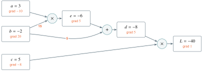
The running example , drawn as a computation graph. Black numbers flow forward (inputs to output). Orange numbers flow backward: each is , how much moves per unit nudge of that value. Because is used twice, it collects 15 along one path and 5 along the other: 20.
Five ideas carry this module.
- Training asks one question per knob. A neural network is a big expression with adjustable numbers called parameters. Training asks, for each one: if I turn this knob a little, does the error go up or down, and how fast? That is a derivative, one per knob.
- A partial derivative freezes the other inputs. With many inputs, take the ordinary Calculus I derivative in one input while treating every other input as a constant.
- Backpropagation is the chain rule, applied node by node. Each operation knows only its own local derivative. It multiplies the gradient arriving from the output side by that local derivative and passes the result to its inputs. A value used in two places adds what arrives from both.
- Order matters. A node may pass its gradient on only after every node that uses it has reported. That order is a reverse topological sort.
- Gradient descent turns gradients into learning. Nudge every parameter a small step against its gradient, then repeat. A finite-difference check proves the gradients are right.
What you will build. About 150 lines of Python in the companion code’s ai-lab/m01_autograd folder: engine.py (the Value class and its backward pass), gradcheck.py, nn.py (neurons, layers, networks), and train.py. Seventy tests check them step by step. At the end, a network you wrote learns XOR, a function no single straight line can separate. A companion-code tool, ai-lab/tools/viz.py, animates your own engine’s backward pass, and the Gradient Explorer on the companion website (bezhig.com/book/explorers/ai01-gradient-explorer.html) lets you drag the learning rate, the finite-difference step, and a neuron’s input and watch what happens.
| Session | Work | Where |
|---|---|---|
| 1 | Warm-up; the question autograd answers; partial derivatives | 1, 2.1–2.2; AI01.01–02 |
| 2 | The chain rule on a graph; adding gradients | 2.3–2.4; AI01.03–05 |
| 3 | Topological sort, gradient descent, finite differences | 2.5–2.7; AI01.06–08 |
| 4 | Python for a C++ engineer; lab steps 1–2 | 2.8; 3.0–3.2 |
| 5 | Lab steps 3–4 and the backprop animation; the bug field guide | 3.3–3.4; 2.10 |
| 6 | Lab steps 5–6 | 3.5–3.6; AI01.09–11 |
| 7 | Lab steps 7–8: train XOR; design trade-offs | 2.9; 3.7–3.8; AI01.12–14 |
| 8 | Code-reading drill, mastery gate, development log | 4.2–4.3; 5 |
2. Deep explanation#
2.1. The question autograd answers#
Here is the smallest network worth the name: one neuron. It takes two inputs and , multiplies each by a weight, adds a bias, and squashes the result:
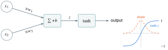
One neuron. The weights and the bias are the knobs. The function (blue) squashes any number into the range to . Its slope (dashed orange) is 1 at and nearly 0 once is far from 0, which is where learning stalls (AI01.09).
The function (the hyperbolic tangent) is defined by . It is an S-shaped curve with that levels off at for large and at for very negative . You will derive its derivative in AI01.09.
The inputs come from data. The weights and and the bias are the knobs, called parameters, and training chooses them. To judge a choice we need one number that says how wrong the network is, the loss. For one example with target , a common loss is the squared error . Training means changing , , and to make smaller.
For each knob the useful question is: if I nudge this knob up a little, how much does change? That is the derivative of with respect to that knob. A real model has millions or billions of knobs. Autograd (automatic gradient) computes every one of those derivatives with one forward pass and one backward pass. That is the machine you build in this module.
2.2. Partial derivatives: freeze the others#
In Calculus I every function had one input. A loss has many. The fix is almost disappointingly simple: to see how changes with , hold every other input fixed. Then is an ordinary one-input function of , and you take its ordinary derivative.
Worked example. Let at the point . First, .
: freeze . Then is a constant multiplier on , and is a constant term whose derivative is :
: freeze . Then is a constant coefficient on :
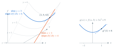
Left: the surface over the -plane. Freezing slices it along the blue curve; freezing slices it along the orange line . Right: the blue slice is an ordinary Calculus I graph, , whose tangent at has slope 6. A partial derivative is the slope of a slice.
The gradient. Collect all the partial derivatives into one list: , read “grad .” At it is . For training we use it one entry at a time: each entry tells its own knob which way to turn and how strongly. (Calculus III proves that the whole list, read as an arrow, points in the direction of steepest increase.)
Small nudges add up. For small nudges and ,
Each partial predicts the change caused by its own nudge, and the two predictions add. This is the tangent-line approximation of Module 13, with one slope per input. Check it: move from to . The prediction is , so . Exactly, . The error, , is far smaller than either nudge. This “add the effects of small nudges” rule is the whole reason backpropagation works (section 2.4).
Check yourself: for the same , what is at ? (Answer: .)
A common misreading. “Freeze ” does not mean stops mattering. The partial derivative still contains : at the slope in is 6, and at it would be 10. Freezing is about which input you nudge, not which inputs the answer may depend on. That is why backprop needs every value from the forward pass.
Say it back (one sentence, out loud or on paper): what does at promise about when moves from 3 to 3.01?
2.3. The chain rule on a graph#
Computation graphs. Any expression can be drawn as a graph. Each node is one value. An arrow from to means “ was used to compute .” The inputs are the leaves, and the last node is the output. The running example with , , builds three nodes (the figure in section 1): , then , then . These are the Russian nesting dolls of composition laid out flat, one node per doll.
Local derivatives: the Modular Workbench. Each node knows only how its own output moves when one of its inputs moves, with its other inputs frozen. These are partial derivatives of a tiny function, and there are only a handful of kinds:
| Node | Local derivative with respect to each input | In words |
|---|---|---|
| , | passes the gradient through | |
| , | each input gets the other one | |
| ( a number) | the power rule; watch the sign of | |
| , which is out itself | ||
| derived in AI01.09 | ||
| (ReLU) | if , and if | at exactly is a convention |
Treat these like , , , in the product rule: find each local derivative on its own line, check it, and only then assemble.
The chain rule, graph form. In Calculus I, if depends on and depends on , then . On a graph this becomes one rule applied at every node:
The upstream gradient is how much the final output cares about this node; your code stores it in the node’s grad. The backward pass starts at the output with : nudging changes by exactly the nudge. That 1 is called the seed.
Worked backward pass for the running example. Work from the output back toward the leaves.
| Step | Node | Upstream | Local derivatives | Sent to inputs |
|---|---|---|---|---|
| 1 | ; | gets ; gets | ||
| 2 | and | gets ; gets | ||
| 3 | ; | gets ; gets |
So and . The leaf received two messages, 5 and 15; the next section shows why they add to . Check algebraically: , so , , and .
Your turn: a faded example. Take at , , with one inner node , so . Fill in the blanks on paper before reading on.
| Step | Node | Upstream | Local derivatives | Sent to inputs |
|---|---|---|---|---|
| 1 | ; | gets ; gets | ||
| 2 | and | gets ; gets |
Then total each leaf. Check after you finish: gets 2 and gets 5; the add node passes 2 to both. So and . Algebra agrees: gives and . Notice that is used twice, which is the subject of the next section.
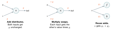
Three patterns cover most of backpropagation. Here is the gradient arriving at the node from the output side.
2.4. Used twice? Add the gradients#
Why should ’s two messages add? The nudge rule from section 2.2 answers it. The node depends on twice: directly, and through . Nudge by a small amount and follow both effects:
- changes by ;
- changes by both: ;
- changes by .
So : one term for each path from to . Check with numbers: gives , a change of .
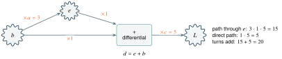
The chain rule as a gearbox. Each local derivative is a gear ratio: turn by one notch and turns 3 notches, because . Along a path the ratios multiply. Where two paths meet at an add node, their turns add, the way the differentials in old mechanical computers added two shafts’ rotations.
In general, is the sum, over every path from to , of the product of the local derivatives along that path. Backpropagation computes exactly that sum without listing the paths. That matters: a graph can have exponentially many paths (a chain of diamonds like the one in lab step 3 has ), yet backprop touches each edge once, because each node stores its total so far and hands it on. Reusing stored partial totals instead of recomputing them is called dynamic programming, a technique Module 3 makes central.
Say it back: using the gearbox picture, explain in two sentences why is 20 and not 15.
The smallest example is at . The multiply node sees the same value on both inputs. It sends “the other input times ” to its first input and to its second input, and both are : at . With = you would get 3. Lab step 4 has you break your own code this way and watch it happen.
2.5. The order of work: topological sort#
A node’s gradient is finished only when every node that uses it has sent its message. In the running example, ’s gradient is not complete until both and have reported. So a node may run its backward step only after all of its users have run theirs.
An ordering in which every node comes after all of its inputs is called a topological order. The forward pass already happens in one. The backward pass runs in the reverse of one: output first, and each node before its inputs.
The algorithm: depth-first search, post-order.
- To visit a node : if has not been visited, mark it visited, visit each of its inputs, and then append to the list.
- Visit the output.
Because is appended only after all of its inputs, every node lands after its inputs. Reverse the list and every node comes before its inputs.
Trace on the running example (children visited in the order for ; for ; for ): visit visit visit visit (append ) visit (append ) append visit again (already visited, skip) append visit (append ) append .

The post-order list for the running example, and the direction the backward pass walks it.
Say it back: why may not run its backward step before has run its own?
The visited set is what stops from being appended twice. That would be harmless for a leaf, but a shared interior node listed twice would run its backward step twice and double-count its gradient (bug B5).
Cost. Every node and every edge is touched once, so the sort is for nodes and edges: proportional to the size of the graph. The whole backward pass costs a small constant multiple of the forward pass, however many inputs there are. (In an engine like yours it is even cheaper than the forward pass: for a 100,000-operation chain on one desktop PC, a complete engine of this design took about 0.06 s for the backward pass, while building the graph took 0.08 to 0.2 s.) That is why training is affordable at all.
A Python limit. Python stops a chain of nested function calls at about 1000 by default (python -c "import sys; print(sys.getrecursionlimit())" prints 1000 on a standard Python installation). A recursive visit on a 5000-node chain therefore raises RecursionError. Stretch S1 replaces the recursion with an explicit stack.
2.6. Gradient descent: turning gradients into learning#
Now use the gradients. Take a knob with gradient . If , increasing increases , so decrease . If , increasing decreases , so increase . Both cases say the same thing: step against the gradient.
The Greek letter (eta) is the learning rate, a small positive number you choose. Updating every knob once is one step.
Why not set and solve, the way calculus finds a minimum (Modules 13 and 14)? For one knob you could. For millions of knobs tangled together through , no formula exists. Walking downhill works anyway.
Worked example. has its minimum at , and . Start at with :
To see the pattern, subtract 3 from both sides of the update:
The distance to the minimum is multiplied by at every step. With that factor is : a steady approach. With it is : the first step lands exactly on 3. With it is : each step overshoots to the other side, by less each time. With it is : the steps bounce between 0 and 6 forever. With the factor’s size exceeds 1, and every step overshoots further than the last.
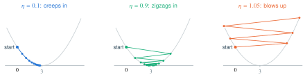
Gradient descent on from . Too small is slow, too large explodes, and the safe range depends on how sharply the loss curves. With many knobs you find a good by experiment (Module 2 runs a learning-rate sweep).
Two knobs at once. With two knobs the loss is a surface, and a contour map shows it from above: each closed curve joins points of equal loss, like the height lines on a hiking map. The gradient points straight uphill, at right angles to the contour through your position, so the update steps straight downhill. (Calculus III proves the right angle; the figure below lets you see it.)
Take . Its gradient is : the bowl is 8 times steeper in the direction. Each knob gets its own factor, exactly as in the one-knob example: and . The steep direction limits the learning rate: converges only when , that is, . At the factor is , so the path zigzags across the valley. At nothing zigzags, but moves only 5% of its remaining distance per step, so progress along the valley floor is slow.
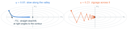
Gradient descent on from . Both axes use the same scale, so the right angle between the downhill arrow and the contour is real. A bowl much steeper in one direction than another is called ill-conditioned. Its steepest direction caps the learning rate, and its gentlest direction then crawls. Optimizers such as Adam (Module 2) give each knob its own effective step size, partly to fix exactly this.
Real losses have many valleys, and gradient descent finds a nearby low point, not necessarily the lowest. For neural networks this works far better than early theory predicted, which is one of the field’s genuine surprises.
Where this goes: every model at Anthropic, OpenAI, and Tesla trains with this loop. The differences are scale: tensors instead of single numbers, GPUs, and smarter step rules such as AdamW (Module 2).
2.7. Checking gradients with finite differences#
How do you know a backward pass is right? Go back to the definition of the derivative, Module 08’s difference quotient, with a small instead of a limit:
For a partial derivative, nudge one input and freeze the others.
Why central is better, Algebra First. Take and expand .
- Forward: . The error, , shrinks in proportion to .
- Central: , so . Dividing by gives . The error, , shrinks in proportion to : the terms cancel because the two nudges are symmetric.
At with the true slope is 12. The forward difference gives 12.61 and the central difference 12.01 (AI01.08).
Why not use a tiny ? A computer stores about 16 significant digits (a Python float is a 64-bit double, with relative precision about ). When is tiny, and agree in almost every digit. Subtracting cancels the digits that agree and leaves mostly rounding noise, and dividing by a tiny magnifies that noise. So rounding error grows like while the approximation error shrinks like or .
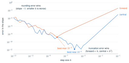
Error in the estimated slope of at , both axes logarithmic. On the right, the approximation error dominates (slope 1 for forward, 2 for central). On the left, rounding error dominates and gets worse as shrinks. The central difference is most accurate near , with an error around ; the forward difference is best near , around .
The Gradient Explorer’s third panel draws this curve live in your browser; slide and watch the error fall, bottom out, and climb again. Practical rule: use the central difference with between and , and compare with a tolerance of about times the size of the gradient. AI01.16 derives the best with Module 14’s optimization. Gradient checks are to autograd what unit tests are to any other program: too slow for training (two evaluations per input), perfect for tests.
2.8. Python for a C++ engineer: exactly what this lab uses#
| C++ | Python in this lab |
|---|---|
| A class with declared members | Members are created by assigning self.data = ... inside __init__. self is an explicit this. |
operator+ overload | def __add__(self, other). Methods named with double underscores (“dunder” methods) are hooks Python calls for operators: __mul__, __pow__, __neg__, __sub__, __truediv__. |
| Overload chosen by type at compile time | For 2 + a, Python first calls the int’s __add__, which returns NotImplemented because it has never heard of Value; then it tries the reflected a.__radd__(2). Without __radd__ you get TypeError. Careful: __rsub__ must compute , not . |
A lambda capturing by reference, [&] | A def nested inside a method is a closure: it remembers self, other, and out from the enclosing call and reads them when it runs later. That is exactly what _backward needs. One trap: closures created in a loop all see the loop variable’s final value (late binding). This lab doesn’t hit it, but remember it. |
A std::function member | Assign a function to an attribute: out._backward = _backward. |
Pointer comparison p == q | a is b. Plain == calls __eq__, which compares identity unless you define it. Define __eq__ and Python removes the default hash, so the class can no longer go in a set (bug B10). Keep Values compared by identity only. |
std::unordered_set<Value*> | set(), which hashes objects by identity by default. |
dynamic_cast check | isinstance(other, Value), used to wrap plain numbers in a Value. |
std::accumulate(first, last, init) | sum(items, start). Without start, sum begins at the int 0, so its first addition is 0 + Value, which needs __radd__. |
double | float is always a 64-bit double. |
| Stack size you can raise | A recursion limit of about 1000 nested calls. |
std::format | f-strings: f"Value(data={self.data}, grad={self.grad})". |
2.9. Design trade-offs: why this design, and what breaks at scale#
- Scalars versus tensors. Your engine stores one number per
Value, and every operation allocates a Python object and a closure. Measured with a complete engine of this design on one desktop PC, one operation costs about 1.5 to 3 microseconds (forward plus backward; building nodes is the slow, variable part) and about 860 bytes of memory. One matrix multiplication, a routine step in a small language model, is multiply-adds, or about of your nodes. At that rate it is two to five days of computing and 118 terabytes of memory. A GPU does it in a few milliseconds. A tensor library stores millions of numbers per node: one matrix-multiply node replaces millions of your nodes and runs on the GPU. The chain rule and the topological sort are identical. Module 2 makes that move. This scale is for understanding, not speed. - Memory. The graph keeps every intermediate value alive until the backward pass, because local derivatives need them (a multiply node needs both inputs’ data). That is why training uses far more memory than running a model. Large models trade compute for memory by recomputing some intermediates during the backward pass, which is called activation checkpointing.
- Built as it runs, or compiled first. Your graph is built by ordinary Python as it runs, so any
iforforworks and an error points at your own line. PyTorch’s default mode works the same way. Compiled approaches such astorch.compileand JAX trace the graph first and then optimize it: faster, harder to debug. Module 2 uses both. - Reverse mode versus forward mode. One backward pass gives the gradient of one output with respect to every input. Forward mode (W04’s dual numbers) carries the derivative with respect to one input forward per sweep, so it needs one sweep per input. One loss and a billion knobs means reverse mode (AI01.15).
- Accumulating gradients is a feature. Because backward adds into
grad, gradients from several backward calls sum. Large-model training uses this to add up gradients over several small batches (“gradient accumulation”). The price is that you must zero the gradients before each step (bug B8). PyTorch does the same for parameters. - The order of addition changes the last digits. Floating-point addition is not exactly associative: and can differ in the last bit, because each sum is rounded. If
_prevwere a set, Python would order the inputs by memory address, which changes from run to run, so gradients would be summed in a different order each time. Usually that is invisible. In training, though, tiny differences can grow. With a set, XOR runs of a complete engine gave a different final loss on every rerun for all 50 random starts tried; in one batch of five reruns, a single start ranged from to . A tuple fixes the order and makes every run identical, which Module 5’s experiment loop depends on. (GPU libraries face the same issue at a much larger scale, and offer “deterministic” modes that trade speed for identical results.) - A closure per node, or a table of operations. Storing a closure in each node is short and flexible. PyTorch instead records which operation made each node and calls a compiled backward function for that operation, which is faster and uses less memory per node.
2.10. Beginner bugs: a field guide#
These are the mistakes people really make when they first write an autograd engine. Each has a symptom you can recognize and at least one test in your lab that catches it. Each was planted, one at a time, in a working engine, and every one of these “mutants” fails at least one of the lab’s tests (AI00, section G).
| Bug | Symptom | How to spot it; which test catches it | |
|---|---|---|---|
| B1 | Overwrite: grad = instead of += | Right answers until a value is used twice; gives 1. The bug can even hide: if the add node overwrites first and a later node adds, the total comes out right. | Test graphs with reuse. In multiply: step 2’s manual backprop. In add: step 4’s test. |
| B2 | Mirror: multiply sends an input its own value | comes out as | Use and check both. Step 2’s multiply test. |
| B3 | Missing seed | Every gradient is 0 | Print the output’s grad. Step 3. |
| B4 | Wrong order: forward order, or appending a node before its inputs | Gradients 0 or partial in deep graphs | A long chain. Step 3’s chain test. |
| B5 | Double visit: no visited set | A shared interior node is counted twice | An interior node used several times. Step 3. |
| B6 | Wrong local derivative: , a dropped minus in , for | Powers wrong, especially negative ones: gets slope instead of | Test negative and fractional exponents, and points away from 0 (at , and agree). Step 5; step 6’s random graphs. |
| B7 | Forgotten chain: local derivative without * out.grad | Correct when the operation is the output, wrong inside a longer expression | Test operations inside a chain. Every step 5 test multiplies by 3 for this reason. |
| B8 | Stale gradients: no zero_grad | Training is erratic or diverges | Loss curve; step 8’s stale-gradient test. |
| B9 | Uphill step: p.data += lr * p.grad | Loss rises every step | Loss curve. Step 8. |
| B10 | Unhashable Value: defined __eq__ | TypeError: unhashable type | The traceback. Step 1. |
| B11 | Reflected operations backwards: computed as | Sign errors whenever a plain number is on the left | Step 5’s rsub and rdiv tests. |
| B12 | Overflowing : computed as | OverflowError for large inputs (math.exp overflows just past 709) | Extreme inputs. Step 5’s saturation test. |
3. The lab: build it yourself#
3.0. Setup and ground rules#
Everything lives in the companion code’s ai-lab/m01_autograd folder; copy the ai-lab folder into a repository of your own first (AI00, section G). You write engine.py, gradcheck.py, nn.py, and train.py; each starts as a set of docstrings that are its specification. The tests folder and check.py come with the starters; don’t edit them. Open a terminal (PowerShell on Windows) in the folder that holds your copy and run the first check:
cd ai-lab\m01_autograd
python check.py 1
Every test fails with “not written yet”. That is the starting line.
- Type the code yourself. Don’t paste from this book or anywhere else: typing is how your hands learn the patterns.
- Predict before every run, in writing. The orange boxes tell you what to predict.
- When a test fails, read the test before your code. Its name says what it checks, and its body in
tests/shows the exact inputs. Reading someone else’s test code is code-reading practice too. - Stuck? Climb that step’s hint ladder (after the practice set, on its own page) one rung at a time.
- Checking your work. The tests are the judge: a step is finished when its tests pass on code you typed yourself. When one fails, find the first incorrect step before you change anything, and log it with its field-guide number (section 2.10). After all eight steps pass, the code-reading drill (section 4.2) compares your engine with micrograd, a complete published engine of the same design.
3.1. Step 1: a Value that remembers where it came from (worked example)#
Goal. A Value holds a number and a gradient and remembers its inputs; + and * build new Values. Type this into engine.py, replacing the matching stubs:
    def __init__(self, data, _children=(), _op="", label=""):
        self.data = float(data)
        self.grad = 0.0
        self._prev = tuple(_children)
        self._op = _op
        self.label = label
        self._backward = lambda: None

    def __repr__(self):
        return f"Value(data={self.data}, grad={self.grad})"

    def __add__(self, other):
        other = other if isinstance(other, Value) else Value(other)
        out = Value(self.data + other.data, (self, other), "+")
        return out
Line by line: float(data) stores a float even when you pass an int. grad starts at 0 because nothing is known yet. _prev holds the inputs, in order, as a tuple. (For a * a it holds a twice; the visited set in step 3 makes sure a is still processed once.) A tuple keeps every run identical to the last digit; section 2.9 explains why a set would not. _op and label are for pictures and debugging. _backward starts as a function that does nothing, which is right for a leaf; every operation will replace it. In __add__, the first line wraps a plain number so that a + 1 works.
Now write __mul__ yourself. It has the same shape as __add__. Only the arithmetic and the operation symbol change.
Run python check.py 1. Passing proves the forward arithmetic, the graph bookkeeping, the wrapping of plain numbers, and that a Value can live in a set.
3.2. Step 2: local backward functions (partly filled)#
Goal. Each operation attaches a _backward that multiplies its local derivatives by out.grad and adds the results into its inputs’ gradients. Extend __add__ and fill in the two blanks from the table in section 2.3:
    def __add__(self, other):
        other = other if isinstance(other, Value) else Value(other)
        out = Value(self.data + other.data, (self, other), "+")

        def _backward():
            self.grad += ____ * out.grad    # d(out)/d(self) for out = self + other
            other.grad += ____ * out.grad   # d(out)/d(other)
        out._backward = _backward
        return out
_backward is defined inside __add__ so that it is a closure: it remembers self, other, and out, and it runs later, once out.grad is known. Now give __mul__ its _backward on your own. Then run the backward pass by hand in the Python prompt:
from engine import Value
a, b, c = Value(3.0, label="a"), Value(-2.0, label="b"), Value(5.0, label="c")
e = a * b; d = e + b; L = d * c
L.grad = 1.0
L._backward(); d._backward(); e._backward()
print(a.grad, b.grad, c.grad)Run python check.py 2.
3.3. Step 3: backward() for the whole graph (on your own, from the recipe)#
Goal. L.backward() fills in every gradient in one call. No code this time: use the recipe in section 2.5 and the three numbered steps in the docstring (sort, seed, walk in reverse). Use a set of visited nodes, and let the output’s gradient with respect to itself be 1.
Run python check.py 3. Then watch it work with the companion code’s visualizer, from the same folder:
python ..\tools\viz.py exampleThis builds the running example with your engine and opens out/graph.html, an animation of the forward pass and then of backprop, one node at a time. It replays your own _backward functions. Step through and watch receive when reports and when reports. If a gradient looks wrong in the animation, the frame where it goes wrong names the operation to fix.
3.4. Step 4: break it on purpose#
This step is an experiment, not new code.
- In
__add__’s_backward, change both+=to=. Predicta.gradafter(a + a).backward()with . Runpython check.py 4and note which tests fail. Restore the+=. - Do the same in
__mul__and predicta.gradfor(a * a).backward()at . Run, note, restore. - Write one sentence in your log: why does
=give exactly 1 for ?
Run python check.py 4 once more with everything restored; all four steps should pass.
3.5. Step 5: the remaining operations (on your own)#
Goal. __pow__, __neg__, __radd__, __sub__, __rsub__, __rmul__, __truediv__, __rtruediv__, exp, tanh, and relu. Their docstrings give the contracts. Before typing each one, write its local derivative on paper (the Workbench).
Build from what you have. An operation made out of existing operations needs no _backward of its own, because the pieces already have one. For example , , and . The trade-off: more nodes (slower) in exchange for less code and fewer places for bugs. __pow__, exp, tanh, and relu need their own _backward. If your power rule drops the sign of the new exponent, check.py reports -48.0 != -0.75 in test_pow_negative_exponent. That is not a coincidence you should shrug at: it is the test’s where belongs, the same slip as answering warm-up question 1 with .
Run python check.py 5.
3.6. Step 6: a gradient checker (on your own)#
Goal. numerical_grad and max_grad_error in gradcheck.py, following section 2.7 and the docstrings. Step 6 also includes a test that builds 40 random expressions from all of your operations and compares your backward pass with central differences computed by the test itself. It is the strongest single check in the lab.
Run python check.py 6.
3.7. Step 7: neurons, layers, networks (partly filled)#
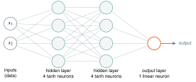
MLP(2, [4, 4, 1]). Every line is a weight. Each neuron also has a bias. Hidden layers apply ; the last layer does not, so the output can be any number.
Goal. nn.py: a Neuron computes (or the plain sum when nonlin=False); a Layer is a list of neurons reading the same inputs; an MLP (multilayer perceptron) applies layers one after another with a linear last layer. Everything is ordinary Python on top of Value, with no new calculus. Here is the neuron with its two key lines left blank:
class Neuron(Module):
    def __init__(self, nin, nonlin=True):
        self.w = [Value(random.uniform(-1, 1)) for _ in range(nin)]
        self.b = Value(0.0)
        self.nonlin = nonlin

    def __call__(self, x):
        act = ____        # w0*x0 + w1*x1 + ... + b, as one Value
        return ____       # tanh of it, unless nonlin is False
Then write Neuron.parameters, Module, Layer, and MLP yourself.
Why random starting weights? If every weight started equal, every neuron in a layer would compute the same thing and receive the same gradient, forever. Random starts break that symmetry. The bias can start at 0 because the weights already make the neurons different. Why a linear last layer? So the output is not trapped between and ; the loss decides what scale it needs.
Run python check.py 7.
3.8. Step 8: teach it XOR (on your own)#
XOR’s output is (blue) when exactly one input is 1, and (red) otherwise.
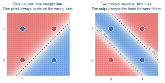
Why XOR needs a hidden layer. Left: one neuron is blue on one side of a straight line and red on the other, and no straight line can put both blue points on one side and both red points on the other. Right: a network wired by hand with two hidden neurons, and , and output . It gives , , , and at the four corners.
Why a hidden layer works. A neuron outputs nearly on one side of the line and nearly on the other, so each neuron draws one soft straight line. On its own it can only split the square into two half-planes. Two hidden neurons draw two lines, and the output neuron adds their votes, so it can keep just the band between them. Training finds weights like the hand-wired ones by itself. Stacking layers this way, building complicated regions out of simple pieces, is the core idea behind deep networks.
Goal. In train.py: mse_loss (the mean of the squared errors), train_step (zero the gradients, forward, backward, update, in that order, returning the loss as a float), and train (repeat, collecting the losses).
Run python check.py 8. Then train and look:
python train.py
python train.py --viz
The second command opens out/xor.html: your loss curve and a map of what your network outputs over the whole input square.
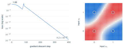
A complete solution’s run with seed 1: MLP(2, [4, 4, 1]), learning rate 0.1, 400 steps of full-batch gradient descent (every step uses all four examples). Left: the loss on a logarithmic scale. It keeps falling at a steady rate (a straight line on this scale) because a network with a linear output can fit four points exactly; on real data the loss levels off instead. Right: the trained network’s output over the input square (blue near , red near , pale near 0), with the four training points. Your curve will differ in detail, because random starting weights depend on how your code draws them.
The spike is not a bug. In that run the loss falls to about by step 74, then shoots up to 2.87 at step 84, higher than where it started, and then falls again. Near the bottom of this valley the loss curves much more sharply than it did at the start. A learning rate that was safe on the gentle early slope is now too big, which is section 2.6’s bounce, happening in 37 dimensions at once. The overshoot throws the weights somewhere flatter, and descent resumes. In runs of a complete solution at learning rate 0.1, 16 of 50 random starts climb back above a loss of 1 after first falling below 0.01 (the worst reaches 6.9), and all 50 still learn XOR. If your curve spikes, check the loss on the steps after the spike before suspecting your code; a smaller learning rate such as 0.05 removes the spikes but learns more slowly.
This is not a toy curiosity; researchers study it directly. As training goes on, the loss surface around the weights often gets sharper (progressive sharpening), and once its sharpest curvature passes ( here), a gradient-descent step overshoots, exactly as in the one-knob example. Cohen et al. (2021) documented this “edge of stability” in full-batch gradient descent. A blow-up that ends in a flatter region also resembles what Lewkowycz et al. (2020) call a catapult, which they observed at the very start of training with a large learning rate. Your spike is consistent with this picture, and stretch S6 shows how you could test it.
When python check.py reports all eight steps passing, you have written a working autograd engine and trained a neural network with it. Copy the summary line into the development log (section 5).
4. Practice, code reading, and the gate#
4.1. Practice set#
F = foundation; C = standard; T = transfer; S = optional stretch; L = lab; R = code reading; G = mastery gate. Follow the session plan in section 1. Attempt each problem completely before opening its solution, and log every miss in error_log.csv with its friction family.
Let . Find and , then evaluate both at . Say which letter is frozen before each derivative.
Which letter is the variable? Let with data and . Find and at , . Name the constants first.
(a) From memory, write the local derivatives of , , , , and with respect to each input. (b) Rewrite as and find and at . Final sweep: check the sign of every exponent.
Draw the graph of with nodes and . At , do the forward pass, then backpropagate by hand with a table like the one in section 2.3. Explain the value you get for , then check all three gradients by expanding .
Build as , using two multiply nodes. At , backpropagate by hand and show that arises as a sum over paths. How many paths lead from to , and what does each contribute?
Algorithm lane. Run the depth-first search of section 2.5 on the running example, but visit each node’s inputs in the opposite order (: then ; : then ; : then ). Give the post-order list and its reverse. Then decide whether each is a valid topological order: (i) ; (ii) ; (iii) .
Gradient descent on from . (a) Take three steps with . (b) Show that . (c) For which does it converge, bounce forever, or diverge? (d) Which reaches 3 in one step?
For at with , compute the forward and central differences and their errors. Then use the expansions in section 2.7 to explain both errors exactly.
Starting from , use the quotient rule to show that . Evaluate it at and at . What does the value at mean for a neuron whose input sum is large?
The sigmoid is . Rewrite it as a power, differentiate, and show that . Evaluate .
One neuron, one step. Let , , and with , , , . Compute the forward pass; then , , , and ; then one gradient-descent step with and the new loss. Give six decimals.
A game engine’s skeleton. In the author’s FateMMO engine, the function that poses a cutout animation rig, evaluatePose, computes a bone’s world scale as its parent’s world scale times its local scale, and its local scale as its bind scale times the animation delta’s scale. Take a chain root arm hand with every bind scale 1, rig-root scale 1, and delta scales , , . (a) Draw the graph for the hand’s world scale and compute . (b) Backpropagate to find , , and . (c) In the same function, world rotation composes by addition. What is the derivative of the hand’s world rotation with respect to the arm’s delta rotation? (d) To make , minimize over alone: take one gradient step with and give the new and loss. (e) In what order would backpropagation visit the bones, compared with evaluatePose’s loop?
Complete lab steps 1–8 until python check.py reports every step passing on your own code. Record the first test that failed and its first incorrect step in error_log.csv.
Mutation hunt. Make each change below in engine.py, one at a time. For each, predict which step’s tests fail first, run python check.py, compare, and undo the change. (a) = instead of += in __mul__; (b) no seed; (c) walk the topological order forwards instead of reversed; (d) ’s local derivative written as ; (e) __rsub__ returning self - other. Write one sentence per change on what the failing test’s name told you.
Reverse mode versus forward mode. A function has inputs and one output, and one evaluation costs . Estimate the cost of all partial derivatives by (a) central differences, (b) forward mode, which needs one sweep per input at a small multiple of each, and (c) reverse mode. Compare for . When would forward mode win?
The best step size. For the central difference, the approximation error is about with (Calculus II’s Taylor series proves this; for you saw exactly ), and the rounding error is about with when is near 1. Minimize with Module 14’s method, compute for , and compare with the figure in section 2.7. (If you haven’t reached Module 14: set and solve for . The solution shows why that gives a minimum.)
4.2. Code-reading drill: micrograd#
micrograd, by Andrej Karpathy (MIT license), is the classic hundred-line autograd engine. The engine you built follows the same design, which makes it the gentlest possible first read of someone else’s code. Read the file at this pinned commit; the line numbers below refer to it:
Protocol. Read the whole file once, top to bottom, without stopping (five minutes). Then, for each question, write your explanation in your own words before opening its solution. Describe what the code does, not what you think it should do.
Lines 5–11 and 24–33. (a) What type is _prev, and what does it contain after e = a * a? (b) Lines 29 and 30 each add to a gradient. For a * a, which object does each line update? Explain why the gradient still comes out as although _prev holds a only once.
Lines 54–70. Explain backward() in three sentences: what build_topo produces, why line 68 exists, and why line 69 uses reversed. Which part would fail on a 5000-node chain, and what error would you see?
Line 68 assigns the seed, while every closure adds. On the running example, predict a.grad, b.grad, and c.grad after calling L.backward() twice without zeroing. Show the second pass node by node. Why is the answer not simply double the first?
(a) Line 49: what gradient does ReLU pass back when its input is exactly 0? (b) Lines 84–91: list the methods that run, in order, when Python evaluates 2 / a, and draw the nodes they create. Use the nodes to compute the derivative of at .
Compare micrograd with your engine. Find two design differences (for example how the topological sort is written, which operations exist, how data is stored, what happens on a 5000-node chain) and give one advantage of each side for each difference.
4.3. Mastery gate#
Find and for at .
Let , , and , at , . Draw the graph, run the forward pass, backpropagate by hand with a table, and check both gradients algebraically.
A linear neuron with squared error on one example , , starting from , . Compute the loss, both gradients, one gradient-descent step with , and the new loss.
Each _backward below has one bug. For each: name it (field-guide number), give the smallest input you can find that exposes it and the wrong result it produces, and fix it.
# inside __mul__
def _backward():
    self.grad = other.data * out.grad
    other.grad = self.data * out.grad

# inside tanh, where t = math.tanh(self.data)
def _backward():
    self.grad += (1 - t) * out.grad
4.4. Next steps#
- Record the module. Keep a progress log, a spreadsheet or CSV with one row per module: first attempt, gate score, teach-back, tests passing, first error, and next review in seven days. Fill in the AI01 row, and log every miss in
error_log.csv. - Calculus. Module 13’s linear approximation is the nudge rule of section 2.2 with one input; Module 14’s optimization reappears in AI01.16. Both will feel familiar now.
- Module 2 starts from the engine you built: a
Valueholding a whole array instead of one number, and the same chain rule with matrix shapes.
5. Development log entry#
Keep a running file DEVLOG.md at the top of your lab repository. It becomes public evidence of what you built, so write every claim so that a stranger could check it. For this module, one entry:
6. Stretch (optional)#
- S1. No recursion. Rewrite
backward()’s topological sort with an explicit stack of(node, children_done)pairs, and passpython check.py --stretch, which backpropagates through a 5000-node chain. - S2. Why reverse mode wins. AI01.15, then the opening of W04 for forward mode with dual numbers.
- S3. The best step size. AI01.16: Module 14’s optimization, applied to the finite-difference error.
- S4. Second derivatives. Your engine cannot compute : each
_backwarddoes arithmetic on plain floats, so the backward pass leaves no graph behind to differentiate again. Sketch what would change if_backwardbuilt newValues instead. This is what PyTorch’screate_graph=Truedoes, and optimizers that use curvature depend on it. - S5. Port it to C++23 (portfolio). Store nodes in one
std::vectorand refer to them by index, as an arena; record each node’s operation as anenumand switch on it in the backward pass instead of storing closures; sort iteratively. Benchmark nodes per second against your Python engine and write up the measured difference. If you already write C++, it plays to your strengths; either way, it gives Module 2’s argument for tensors your own numbers. - S6. A research question you can already ask (best after Module 2’s vectors). Is the XOR spike a catapult? The prediction: the loss’s sharpest curvature is above just before the spike and below it just after. You can measure it with tools you have. Your engine gives gradients, and a finite difference of two gradients, for a direction of length 1, gives a new vector: how the gradient itself changes as you move along . Re-aim along that vector, rescale it to length 1, and repeat (power iteration). turns toward the sharpest direction, and the vector’s length settles at the sharpest curvature. (Strictly, it finds the largest curvature in size, which near a minimum is the sharpest one.) Plot it next to the loss curve. This is how researchers measure the effect; a clean plot of it on your own engine is a genuine small result worth a write-up.
Frontier connections: where this module’s ideas show up at scale#
Read these after the gate, for orientation. Each links a Module 1 idea to the paper where it matters for large models; later modules return to them.
- Built as it runs (section 2.9). PyTorch’s design paper argues that an eager, define-by-run style like your engine’s can still be fast: Paszke et al. (2019), arxiv.org/abs/1912.01703.
- The graph costs memory (2.9). Recomputing some activations during the backward pass trades one extra forward pass for far less memory: Chen et al. (2016), arxiv.org/abs/1604.06174.
- Rounding (2.7). Large models train in 16-bit or 8-bit numbers, where your rounding-error curve moves far to the right. Loss scaling and a 32-bit master copy of the weights keep training stable: Micikevicius et al. (2017), arxiv.org/abs/1710.03740.
- The ill-conditioned valley (2.6). Adam gives each parameter its own step size (Kingma and Ba, 2014, arxiv.org/abs/1412.6980); AdamW fixes how it handles weight decay (Loshchilov and Hutter, 2017, arxiv.org/abs/1711.05101). Muon, an optimizer developed through the public NanoGPT speedrun, goes further and reshapes each weight matrix’s whole update: kellerjordan.github.io/posts/muon/.
- Initialization and learning rates (3.7, 2.6). Under the right scaling rules, the best learning rate found on a small model transfers to a much wider one, so large runs can be tuned cheaply: Yang et al. (2022), arxiv.org/abs/2203.03466.
- Spikes (3.8). Cohen et al. (2021), arxiv.org/abs/2103.00065; Lewkowycz et al. (2020), arxiv.org/abs/2003.02218.
Hint ladders for the lab#
Climb one rung at a time, and try again after each one. Rung 1 is a question, rung 2 points to the idea, rung 3 is a skeleton with the key parts left for you.
L1. Step 1: a Value that remembers#
Rung 1. Which six attributes does the class docstring promise? List them on paper before typing.
Rung 2. Section 2.8: dunder methods, and isinstance for wrapping plain numbers.
Rung 3. __mul__ is __add__ with two changes: the arithmetic (* for +) and the operation symbol ("*" for "+"). Nothing else changes yet.
L2. Step 2: local backward functions#
Rung 1. For : if you nudge by one unit with frozen, how much does out move?
Rung 2. Section 2.3’s table gives each local derivative; section 2.4 explains why every line uses +=.
Rung 3.
        def _backward():
            self.grad += <d(out)/d(self), using numbers you have> * out.grad
            other.grad += <d(out)/d(other)> * out.grad
        out._backward = _backward
L3. Step 3: backward()#
Rung 1. Which node’s gradient do you know without computing anything? Which node can safely run its _backward first, and which must wait?
Rung 2. Section 2.5: depth-first search, post-order, then reverse.
Rung 3.
        order, visited = [], set()
        def visit(v):
            if ____:
                ____
                for child in ____:
                    visit(child)
                order.append(v)      # why here, and not before the loop?
        visit(self)
        ____ = 1.0
        for v in ____:
            v._backward()
L4. Step 4: break it on purpose#
Rung 1. In a + a, how many times does the add node’s _backward write to a.grad?
Rung 2. Section 2.4, the smallest example.
Rung 3. With =, the line for other runs second, and other is a. What value does it leave behind? Restore += before moving on.
L5. Step 5: the remaining operations#
Rung 1. Can the new operation be written using ones you already have? Which four cannot?
Rung 2. Section 2.3’s table; section 2.8 on reflected operators; the field guide’s B6, B11, and B12.
Rung 3.
    def __pow__(self, n):
        out = Value(self.data ** n, (self,), f"**{n}")
        def _backward():
            self.grad += (____) * out.grad
        out._backward = _backward
        return out

    def __rsub__(self, other):    # other - self
        return ____               # build it from operations you have
For , compute the forward value with a function that cannot overflow (the math module has one), and write its local derivative in terms of out.data.
L6. Step 6: the gradient checker#
Rung 1. To estimate , which coordinates change and which stay fixed? What must xs look like when you return?
Rung 2. Section 2.7: the central difference.
Rung 3.
    grads = []
    for i in range(len(xs)):
        up, down = list(xs), list(xs)      # copies, so xs is never changed
        up[i] += h
        down[i] -= h
        grads.append(____)
    return grads
For max_grad_error, the float version of f is lambda x: f([Value(v) for v in x]).data.
L7. Step 7: neurons, layers, networks#
Rung 1. Which Value operations does need? What does sum start from if you don’t tell it?
Rung 2. Section 2.1’s neuron; section 2.8 on sum(items, start).
Rung 3.
        act = sum((wi * xi for wi, xi in zip(self.w, x)), self.b)
        return ____ if self.nonlin else ____

class MLP(Module):
    def __init__(self, nin, nouts):
        sizes = [nin] + nouts
        self.layers = [Layer(sizes[i], sizes[i + 1], nonlin=____)
                       for i in range(len(nouts))]
In MLP.__call__, remember that a hidden layer of width 1 hands back a single Value, while the next layer’s neurons expect a list. If you see 'Value' object is not iterable, that is the cause.
L8. Step 8: training#
Rung 1. Which four things happen in one step, and in what order? What is in grad before you begin?
Rung 2. Section 2.6 (the update rule), and the field guide’s B8 and B9.
Rung 3.
def train_step(model, xs, ys, lr):
    model.zero_grad()
    loss = mse_loss([model(x) for x in xs], ys)
    loss.backward()
    for p in model.parameters():
        p.data ____ lr * p.grad
    return ____
Complete solutions: AI01#
Open a solution only after you have written your own attempt. Compare at the first step where your work differs. A corrected answer is not yet an independent success.
AI01.01Show solution
Freeze, then differentiate
Freeze : is the constant times , the term is constant, and has derivative 1. So , and at it is . Freeze : is the constant times , gives , and is constant. So , and at it is . Each term that does not contain the active letter disappears.
Back to AI01.01AI01.02Show solution
Data is frozen; knobs vary
The constants are the data, and ; the variables are and . Let (the residual), so . By the chain rule, and . At , : , so and . The factor in is the inner derivative. Forgetting it is the classic slip, and it is exactly “gradient equals twice the residual times the input,” which Module 2 will write for a whole matrix at once.
Back to AI01.02AI01.03Show solution
The Workbench table, then a rewrite
(a) : 1 and 1. : and . : . : . : . (b) . Freeze : . Freeze : . Final sweep: the new exponent is , still negative. Writing or here is the same slip as in warm-up question 1.
Back to AI01.03AI01.04Show solution
Two paths that cancel
Forward: , , .
| Node | Upstream | Local derivatives | Sent |
|---|---|---|---|
| 1 | , | gets , gets | |
| 1, 1 | gets , gets | ||
| , | gets , gets |
Totals: , , . At this point a small nudge to pushes down through exactly as much as it pushes up through . A zero gradient doesn’t mean doesn’t matter; it means its effects balance here. Expanding, , so , , and .
Back to AI01.04AI01.05Show solution
Where the 3 in comes from
Forward: , . Backward: has gradient 1. The node sends the value and sends the value (the direct path). The node has as both inputs, so it sends to its first input and to its second, and both land on . Total: . There are three paths, one for each place appears, and each contributes . That is why the power rule’s coefficient equals the number of copies.
Back to AI01.05AI01.06Show solution
Many valid orders
With the opposite child order: visit visit (append ) visit visit (append ) visit already visited visit (append ) append append append . The post-order is and its reverse is . (i) is valid: follows and , follows and , and follows and . (ii) is valid; it is the list just found. (iii) is invalid: comes before its inputs and . A graph usually has many topological orders, and backpropagation works with any of them.
Back to AI01.06AI01.07Show solution
The factor
(a) , , , as in section 2.6. (b) ; subtract 3 from both sides and factor: . (c) Let . The iteration converges when , that is for (without overshooting when , zigzagging when ). At , and it bounces forever. For , and it diverges. (d) makes . For the factor becomes : the steeper the valley, the smaller the safe learning rate.
Back to AI01.07AI01.08Show solution
Expand, then compare
and . Forward: , error . Central: , error . Section 2.7 predicts both exactly. The forward error is , and the central error is .
Back to AI01.08AI01.09Show solution
and saturation
Let and . Since , we get and . The quotient rule gives
At : , so the derivative is . At : , so it is . A neuron whose input sum is 3 passes back less than 1% of the gradient it receives, so its weights barely learn: it is saturated. Keeping sums in the responsive middle of is the job of good initialization and normalization in Module 2.
Back to AI01.09AI01.10Show solution
Rewrite, differentiate, then clean up the fraction
. Outer layer: . Inner layer: . The product is ; the two minus signs cancel. Now , so . At 0: , so .
Back to AI01.10AI01.11Show solution
One neuron, one step
Forward: , , . Backward: ; ; . Since and , both and equal . Step: and . New forward: , , new loss . One step cut the loss by a factor of 18.
Back to AI01.11AI01.12Show solution
A skeleton is a computation graph
(a) : the root’s world scale is the rig scale times , the arm’s is that times , and the hand’s is that times . So . (b) Start with gradient 1 at . The hand’s multiply sends the arm’s world scale (1) to and to the arm’s world scale. The arm’s multiply sends the root’s world scale times 3, which is , to , and to the root’s world scale. The root’s multiply sends to . So , , : each is the product of the other two scales. (c) World rotations add, and add passes gradients through unchanged, so the derivative is . (d) With , . Then , giving and loss , down from 1. (e) evaluatePose runs root, arm, hand (parent first). Backpropagation runs hand, arm, root: the same list, reversed. Fitting joint parameters to move an end effector toward a target by gradient descent is one standard way to solve inverse kinematics.
AI01.13Show solution
The tests, and the usual first failures
Your own code passing every test is the result; there is no single correct file to match, and section 4.2 compares your design with a published one. The usual first failures, in order: B10 (an __eq__ was defined) in step 1; B1 or B2 in step 2; B3 or B4 in step 3; B6 with negative exponents, and B12, in step 5; B8 in step 8. Log the category and the first incorrect step, not just “fixed.”
AI01.14Show solution
What each mutation breaks
(a) = in __mul__: step 2’s manual backprop fails first, with ’s gradient 15 instead of 20, because ’s report overwrites ’s. (b) No seed: step 3 fails, with every gradient 0. (c) Forward order: step 3 fails; leaves run their (empty) backward first, and the output’s gradient reaches its inputs only after they have already run. Only graphs one operation deep survive (the single-leaf test, the seed test, , and ), because their inputs are leaves with nothing to pass on. (d) : step 5’s test fails, and so do step 6’s random graphs. The saturation test fails too, but only because of : there , so while . At , and both expressions give 0, so a test at alone would have missed it. Test away from special points, and on both sides of them. (e) self - other: step 5’s rsub test fails with -6.0 != 6.0. You computed instead of , and the test multiplies by 3. In each case, the failing test’s name points straight at the idea that broke.
AI01.15Show solution
Reverse mode is why training is affordable
(a) Central differences need two evaluations per input: about . (b) Forward mode needs one sweep per input: about times a small multiple of . (c) Reverse mode needs one forward and one backward pass: a small constant multiple of that does not grow with (it does need memory to keep the graph). For and second, finite differences would take seconds, about 63 years; reverse mode takes a few seconds. Forward mode wins with few inputs and many outputs. With one input and outputs, one forward sweep gives all derivatives while reverse mode needs backward passes, and forward mode stores no graph.
Back to AI01.15AI01.16Show solution
Module 14 applied to a numerical method
. Setting it to zero: , so . With and : . It is a minimum because . The error there is . The figure’s best central step, near with error near , agrees in order of magnitude. Real rounding errors are often smaller than the worst case, and for at 0.5, .
Back to AI01.16AI01.17Show solution
A set of inputs, two separate updates
(a) Line 10 builds _prev as a set of the children. For a * a the children are (a, a), so the set holds a once. (b) In the multiply closure, self and other are both a. Line 29 adds into a.grad, and line 30 adds into the same object again, so a.grad becomes . The set only controls which nodes the traversal visits. The arithmetic lives in the closure, which captured self and other as two separate names. If either line used =, the second would overwrite the first and give (bug B1). Your engine stores the tuple (a, a) instead; the visited set in backward() makes sure a is still processed once, so both designs give the same gradient.
AI01.18Show solution
Sort, seed, reverse
build_topo (lines 59–64) is a recursive depth-first search that appends a node only after all of its children, using the visited set so that each node appears once; the result is a topological order. Line 68 seeds the output’s gradient with 1, because . Line 69 walks the list in reverse, so each node runs its _backward only after every node that uses it has added its contribution. On a 5000-node chain, build_topo calls itself once per node, which exceeds Python’s default limit of about 1000 nested calls and raises RecursionError: maximum recursion depth exceeded.
AI01.19Show solution
Assign the seed, accumulate everything else
After the first call: , , , , , . The second call first resets ’s gradient to 1. Then, in reverse topological order:
- : gains and becomes 10; gains and becomes .
- , now with gradient 10: gains 10 and becomes 15; gains 10 and becomes 30.
- , now with gradient 15: gains and becomes ; gains and becomes 75.
Final: . Doubling would give , , . The interior gradients of and were never reset, so each started the second pass already holding its first-pass value, added a second copy, and passed the inflated total downstream. Only , a direct input of (whose gradient was reset), is exactly doubled. PyTorch avoids this. It refuses a second backward pass through the same graph unless you pass retain_graph=True, and even then it recomputes the gradients through the graph from scratch and only adds the results into the leaves’ .grad, so the leaves would be exactly doubled. The lesson: zero every gradient (or build a fresh graph) before each backward pass.
AI01.20Show solution
A convention, and a chain of fallbacks
(a) Line 49 multiplies the incoming gradient by the truth value of “output greater than 0.” At input 0 the output is 0, so that is false (0) and ReLU passes back 0. The true derivative does not exist at the corner; any value from 0 to 1 is defensible, and 0 is the common convention (PyTorch uses it too). (b) Python first asks the int 2 to divide by a; the int returns NotImplemented, so Python calls a.__rtruediv__(2) (lines 90–91). That computes 2 times a to the power . The power runs first (__pow__, lines 35–43), making node . Next comes the product with the plain number 2. The int again returns NotImplemented, so Python calls p.__rmul__(2) (lines 84–85), which calls __mul__ (lines 24–33). That wraps 2 in a Value (line 25) and makes node . The nodes are , , the wrapped 2, and . Backward: starts at 1; the multiply sends to ; the power sends to . So the derivative is , matching . The exponent stays negative.
AI01.21Show solution
What a good comparison contains
A strong answer names two real differences and gives each side a fair advantage. Typical differences:
- The sort. micrograd’s sort is recursive: short and easy to read, but limited to about 1000 levels. An explicit stack handles any depth but is longer.
- Set or tuple. micrograd’s set stores each input once and is simple, but it orders inputs by memory address, so gradient sums can differ in the last digits from run to run. A tuple costs a duplicate entry for
a * aand gives identical runs (section 2.9). - The operations. micrograd has no
tanhorexpin its engine (its network uses ReLU). A smaller surface means fewer tests; more operations means more places for bugs. - Stored types. micrograd keeps whatever number type it is given (an int stays an int, and gradients start as the int 0). Converting to float keeps printing and arithmetic uniform.
- Power exponents. micrograd checks with an
assertthat the exponent is a plain number. ATypeErroris more conventional in library code, and anassertdisappears entirely underpython -O.
If both your differences are cosmetic (names, comments, formatting), find one that changes behavior.
Back to AI01.21AI01.22Show solution
Gate: freeze, then differentiate
Freeze : is times the constant , and is constant. So , which is at . Freeze : , which is .
Back to AI01.22AI01.23Show solution
Gate: backpropagation by hand
Forward: , , . Backward: gives the gradient . Then sends 6 to and 6 to (first path). Then sends to (second path) and to . Totals: and . Check: , so and .
Teach-back rubric (gate part 3). A complete explanation (i) names both paths from to and what each carries: 15 through (local derivative times 5) and 5 directly into (local derivative 1 times 5); (ii) says the two add because the effects of small nudges add; (iii) says a node’s gradient is complete only after all of its users have reported, which reverse topological order guarantees; and (iv) uses “upstream gradient” and “local derivative” correctly.
Back to AI01.23AI01.24Show solution
AI01.25Show solution
Gate: find the bugs
First snippet: B1, the overwrite. Smallest exposing input: a * a with . Both lines write a.grad, the second overwrites the first, and you get instead of . Any graph where a value has more than one user also exposes it. Fix: += on both lines. Second snippet: B6, a wrong local derivative ( instead of ). At both give 1, so a test at 0 passes. At the code gives instead of . Fix: self.grad += (1 - t**2) * out.grad. Lesson: test away from special points such as 0 and 1.
Warm-up answers#
1. : the new exponent is , still negative. 2. Outer layer , inner layer : . 3. , so .
Retention and readiness#
In two days, redo AI01.04 and AI01.09 without looking. In seven days, make up a fresh backpropagation-by-hand problem in the style of AI01.23 (a new expression and new numbers), solve it by hand, check every gradient with your own engine, and redo AI01.19. Log every miss under its friction family. Move on to Module 2 only after the mastery gate in section 4.3 passes.