Module 38: Multivariable extrema and constrained optimization

8 exercises, each with a complete solution. 1 figure.

On this page

A. Prerequisites and observable goals
B. The central idea: allowed directions determine what an optimum means
C. Interior and constrained tests
D. Why the Hessian and multiplier conditions arise
E. A candidate-comparison workflow
F. Worked examples
G. Independent practice
H. Complete solutions: Module 38
I. Retention and readiness

A. Prerequisites and observable goals#

Before

Gradients, critical points, systems of equations, and single-variable optimization.

After

Classify regular critical points, inspect boundaries on compact regions, and use Lagrange multipliers without losing singular or boundary candidates.

B. The central idea: allowed directions determine what an optimum means#

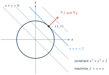
At an unconstrained interior extremum of a differentiable function, every first-order directional change must vanish, so the gradient is zero. Under a constraint, only tangent directions are allowed. The gradient can be nonzero while pointing entirely normal to the constraint, making every permitted first-order change zero. This is the geometric basis of Lagrange multipliers.

At a constrained maximum the level line touches the constraint. To maximize

f=x+y

on the circle

x^2+y^2=2

, slide the level lines

x+y=c

outward. The last one to meet the circle is

x+y=2

, which touches it at

(1,1)

. There the gradients of

f

and of the constraint function

g

point the same way:

\grad f=\lambda\grad g

C. Interior and constrained tests#

For a $C^2$ function of two variables at a critical point, set

D=f_{xx}f_{yy}-f_{xy}^2.

If $D>0$ and $f_{xx}>0$ , there is a local minimum; if $D>0$ and $f_{xx}<0$ , a local maximum. If $D<0$ , the point is a saddle. If $D=0$ , this test is inconclusive. These are local conclusions; global extrema require the domain and boundary to be examined.

A continuous function on a compact region (closed and bounded in Euclidean space) attains maximum and minimum values. To find them, consider interior critical points, boundary curves or surfaces, corners, and any points where differentiability fails.

For a smooth equality constraint $g(\vv x)=c$ , at a constrained local extremum where $\grad g\ne0$ , Lagrange’s necessary condition is

\grad f=\lambda\grad g,\qquad g=c.

It provides candidates, not automatic winners. With multiple regular constraints, the objective gradient is a linear combination of their gradients; independence of constraint gradients matters. Singular constraint points and inequality boundaries need separate treatment. [O3Opt]

D. Why the Hessian and multiplier conditions arise#

At a critical point, the leading local change is governed by the quadratic expression $\tfrac12(f_{xx}h^2+2f_{xy}hk+f_{yy}k^2)$ , with a smaller-order remainder for a $C^2$ function. A positive definite quadratic expression makes all small changes positive; an indefinite one takes both signs and creates a saddle. The determinant test classifies this two-variable quadratic form.

On a regular constraint, tangent directions are perpendicular to $\grad g$ . At an extremum, they must also be perpendicular to $\grad f$ . For a single regular constraint, the normal direction is spanned by $\grad g$ , so the two gradients are parallel. The multiplier is the scale relating them, not a new physical coordinate.

E. A candidate-comparison workflow#

State the feasible region. For an unconstrained problem, solve all partial derivatives equal to zero and check missing-derivative points. Classify with the Hessian only where its hypotheses hold; otherwise inspect signs or higher-order terms. For a compact region, add all boundary candidates before comparing objective values. For a constraint, solve the multiplier equations and the original constraint together, then inspect singular points and boundaries omitted by the regular equations. Confirm the final quantities satisfy the original constraints.

F. Worked examples#

An unconstrained quadratic. For $f=x^2+2y^2-4x+8y$ , the gradient vanishes at $(2,-2)$ . The Hessian has $f_{xx}=2$ , $f_{yy}=4$ , $f_{xy}=0$ , so $D=8>0$ gives a local minimum. Completing squares gives $f=(x-2)^2+2(y+2)^2-12$ , proving it is the unique global minimum, value $-12$ .

A circle constraint. Maximize $f=x+2y$ on $x^2+y^2=5$ . The multiplier equations $(1,2)=\lambda(2x,2y)$ imply $y=2x$ . The constraint then gives $x=\pm1,y=\pm2$ with matching signs. Values are $5,-5$ , so these are the maximum and minimum. Compactness guarantees extrema, and the nonzero circle gradient ensures the regular candidates cover them.

An inconclusive Hessian. The function $x^4+y^4$ has zero Hessian at the origin yet a strict minimum because all nearby nonzero values are positive. The function $x^4-y^4$ has the same zero Hessian there but a saddle. The zero determinant carries no classification by itself.

G. Independent practice#

F foundation C standard course work T transfer S optional stretch L runnable lab or project. Attempt the complete set before opening its solutions.

M38.01FSolution

Find and classify the critical point of $f=x^2+3y^2-2x+6y$ . Determine whether the classification is global.

M38.02CSolution

Find and classify all critical points of $f=x^3-3x+y^2$ .

M38.03TSolution

Classify the origin for $f=x^4+y^4$ and $g=x^4-y^4$ , explaining why the second-derivative test is inconclusive.

M38.04TSolution

Find absolute extrema of $f=xy$ on the rectangle $-1\le x\le2$ , $0\le y\le3$ . Include boundaries.

M38.05CSolution

Use Lagrange multipliers to maximize and minimize $f=3x+4y$ on $x^2+y^2=4$ .

M38.06TSolution

Find the point of the plane $x+2y+2z=9$ closest to the origin. Use a squared-distance objective and verify the constraint.

M38.07TSolution

Among nonnegative $x,y,z$ with $x+y+z=12$ , maximize $xyz$ . Explain why a boundary point cannot be the maximizing point.

M38.08SSolution

Minimize $f(x,y)=x$ subject to $g(x,y)=x^2+y^2=0$ . Show why the feasible point is an optimum even though no multiplier solves $\grad f=\lambda\grad g$ there.

Optional small hints

For M38.02, solve $3x^2-3=0$ and $2y=0$ before classifying. For M38.04, the boundary includes four line segments. For M38.08, inspect the nonzero-gradient hypothesis on the constraint.

H. Complete solutions: Module 38#

Compare the first step where your work differs. A corrected answer is not yet an independent success.

M38.01Show solution

A positive quadratic form gives a global conclusion

The gradient is $(2x-2,6y+6)$ , so the only critical point is $(1,-1)$ . The Hessian test has $D=2\cdot6=12>0$ and $f_{xx}=2>0$ , a local minimum. Completing squares gives $f=(x-1)^2+3(y+1)^2-4$ , proving the unique global minimum value is $\boxed{-4}$ at $\boxed{(1,-1)}$ . There is no global maximum on $\R^2$ .

Back to M38.01

M38.02Show solution

The same equation can have a saddle and a minimum

The gradient vanishes at $(1,0)$ and $(-1,0)$ . Here $f_{xx}=6x$ , $f_{yy}=2$ , $f_{xy}=0$ , so $D=12x$ . At $(1,0)$ , $D>0$ and $f_{xx}>0$ , giving a local minimum of value $-2$ . At $(-1,0)$ , $D<0$ , giving a saddle of value $2$ . The cubic is unbounded above and below, so the local minimum is not a global one.

Back to M38.02

M38.03Show solution

Use sign information when the Hessian vanishes

Both functions have zero first and second partials at the origin, so $D=0$ . For $f$ , $x^4+y^4>0$ whenever $(x,y)\ne(0,0)$ , giving a strict global minimum of zero. For $g$ , the axis values $g(h,0)=h^4$ and $g(0,h)=-h^4$ show both signs arbitrarily nearby, hence a saddle. The inconclusive test is resolved by direct comparison.

Back to M38.03

M38.04Show solution

The best values occur on the boundary

The function is continuous on a compact rectangle. Interior critical equations $y=0,x=0$ yield no interior point because $y=0$ is a boundary. On $y=0$ , $f=0$ . On $y=3$ , $f=3x$ ranges from $-3$ to $6$ . On $x=-1$ , $f=-y$ ranges from $-3$ to $0$ ; on $x=2$ , $f=2y$ ranges from $0$ to $6$ . Thus the absolute minimum is $\boxed{-3}$ at $(-1,3)$ and maximum $\boxed6$ at $(2,3)$ .

Back to M38.04

M38.05Show solution

Solve the parallel-gradient equations and compare values

The equations are $3=2\lambda x$ , $4=2\lambda y$ , and $x^2+y^2=4$ . They force $(x,y)$ parallel to $(3,4)$ with length $2$ , giving points $\pm(6/5,8/5)$ . Their objective values are $\pm10$ . Thus the maximum is $\boxed{10}$ at $(6/5,8/5)$ and minimum $\boxed{-10}$ at the opposite point. The circle is compact and regular, so these candidates suffice.

Back to M38.05

M38.06Show solution

The minimizing vector is normal to the plane

Use $F=x^2+y^2+z^2$ . The multiplier equations give $(2x,2y,2z)=\lambda(1,2,2)$ , so $(x,y,z)=k(1,2,2)$ . The constraint becomes $9k=9$ , so $k=1$ and the point is $\boxed{(1,2,2)}$ . Its distance is $\boxed3$ . For any other feasible point, the displacement from this point lies in the plane and is perpendicular to $(1,2,2)$ , so Pythagoras makes its squared distance $9$ plus a nonnegative term. This verifies the global minimum despite the unbounded constraint set.

Back to M38.06

M38.07Show solution

Check the boundary before dividing by variables

The feasible triangle in the nonnegative octant is compact. Any boundary with one coordinate zero has product zero, while $(4,4,4)$ gives a positive product, so a maximum lies in the positive interior of the constraint. There the equations $yz=xz=xy=\lambda$ imply $x=y=z$ after division by positive factors. The sum constraint gives each equal to $4$ , and the maximum is $\boxed{64}$ . Boundary checking justified the divisions and ruled out missing maximizers.

Back to M38.07

M38.08Show solution

A singular constraint invalidates the regular multiplier test

The only feasible point is $(0,0)$ , so it is both a constrained minimum and maximum, with value zero. But $\grad g(0,0)=(0,0)$ while $\grad f=(1,0)$ . No scalar multiple of the zero vector equals $(1,0)$ . The multiplier theorem’s regularity assumption $\grad g\ne0$ fails, so this is not a contradiction. Singular feasible points require direct inspection.

Back to M38.08

I. Retention and readiness#

Retrieve M14.08 and M37.08. Explain why an interior derivative test cannot replace a boundary search and why a multiplier equation supplies candidates rather than proof of optimality. Complete Mixed Review R3 before beginning multiple integrals.