Derivative sign charts, critical numbers, closed-interval extrema, and basic geometry.
After
Translate derivative signs into graph behavior and solve a constrained optimization problem from a mathematical model.
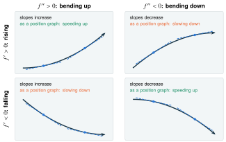
Picture 14.1. The shape alphabet. Every curved stretch of a smooth graph is one of four strokes. The sign of f′ says rising or falling; the sign of f′′ says which way the graph bends, because f′′ is the slope of the slope. Compare the two dashed tangent lines in each cell: from left to right they steepen or flatten. Read as a position graph, this is Module 12’s rule again: when f′ and f′′ have the same sign, the speed grows.
B. The central idea: use derivatives to compare nearby choices#
A function’s height, slope, and bending are different pieces of information. The first derivative describes increasing or decreasing behavior. The second derivative describes how the slope changes. Optimization uses this information after the feasible choices have been expressed as a domain: the best algebraic critical point is irrelevant if it violates the problem’s constraints.
On an interval, f′>0 implies increasing and f′<0 implies decreasing, by the MVT. At a critical input c, a first-derivative sign change +→− gives a local maximum; −→+ gives a local minimum. No sign change means this test does not produce an extremum.
Where f′′>0, the graph is concave up; where f′′<0, concave down. An inflection point is a point on the graph where concavity changes. A zero of f′′ is only a candidate, and a missing domain point cannot be an inflection point of the graph. If f′(c)=0 and f′′(c)>0, the second derivative test gives a local minimum; f′′(c)<0 gives a local maximum. If f′′(c)=0, the test is inconclusive.
An absolute maximum on a closed interval must still be compared against endpoints and all other critical candidates. For an open or unbounded feasible interval, investigate behavior at the ends; do not assume a best value is attained. Standard derivative applications: [O1Apps].
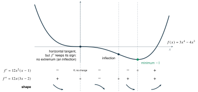
Picture 14.2. From sign chart to sketch. Factor f′ and f′′, mark their zeros on two number lines, write a sign in every gap, and read off one stroke of the shape alphabet per gap. At x=0 the derivative is zero but does not change sign, so there is no extremum there, only a level spot where the bending flips. The only extremum is the minimum at x=1.
If f′ increases, moving right from a produces slopes at least as large as f′(a). The secant slope from a to x>a, by the MVT, is one of those intermediate slopes. Therefore f(x)−f(a)≥f′(a)(x−a), placing the graph above the tangent. The same conclusion holds to the left after the sign of x−a is handled. This explains the underestimate for a concave-up graph in Module 13.
An optimization model often turns many choices into one variable. A rectangle with fixed perimeter cannot change width and length independently. Eliminating one variable is not a calculus trick: it expresses the constraint, and the remaining interval expresses physical feasibility.
For a graph: record domain and intercepts, discontinuities or asymptotes, zeros and undefined points of f′, derivative signs, and concavity. Use those features to construct a coherent sketch rather than drawing a smooth curve through a few sampled points.
For optimization: name the quantity to maximize or minimize; write its units; express it with the constraints; state the feasible domain; find critical inputs; justify the winner globally; and translate the input back into all requested dimensions. If the model is wrong, flawless differentiation solves the wrong problem.
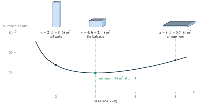
Picture 14.3. The tank trade-off. An open-top tank with a square base must hold 32 m3, and its material is its surface area S(x)=x2+x128, the floor plus four walls. Too narrow and the walls grow tall; too wide and the floor grows huge. Both ends of the domain cost too much, so the best tank is in between, where S′(x)=0: a 4 m square, 2 m deep. The tanks are drawn to one scale.
Curve behavior. Let f(x)=x3−3x. Then f′=3(x−1)(x+1) and f′′=6x. The graph increases on (−∞,−1) and (1,∞) and decreases between. Its local maximum is (−1,2) and local minimum is (1,−2). Concavity changes at (0,0). There is no absolute extremum on all of R because the cubic is unbounded above and below.
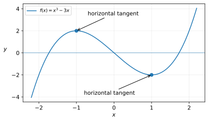
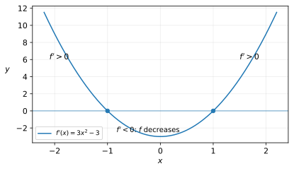
The exact cubic f(x)=x3−3x has slope zero at two nonzero heights. Its concavity changes at zero, where its slope is negative.
A fixed-perimeter rectangle. With perimeter 40 m, length ℓ=20−w. The area is A(w)=w(20−w) for 0<w<20. Then A′=20−2w, so w=10 and ℓ=10. Since A′′=−2<0 everywhere and the area tends to zero at either feasible end, this is the absolute maximum. Equivalently, A=100−(w−10)2≤100 proves the result without calculus and checks it.
Exact derivative graph for the preceding cubic f(x)=x3−3x. Its zeros locate horizontal tangents, and its sign determines the cubic’s increasing and decreasing intervals. A negative derivative means decreasing height, not necessarily negative height.
Optimization problems usually fail in the modelling, not in the calculus. Run them on a workbench, one move per line, just as you ran related rates in Picture 12.4.
Picture and goal. Draw it. Name the quantity to make largest or smallest, with its units.
Objective. Write that quantity using every variable in the picture.
Constraint and domain. Use the constraint to cut down to one variable, then write the feasible domain: every value that makes a real object.
Candidates. Critical points inside the domain, plus the endpoints, or the behavior near an open end.
Prove it is the best, then answer the question. Compare candidates, or read the sign of the derivative around the only critical point. Then report every quantity the question asks for, with units.
Worked example: the tank in Picture 14.3. An open-top tank with a square base must hold 32 m3. Use the least material.
Goal: minimize the surface area S (m2). Base side x and depth h, in metres.
Objective: S=x2+4xh, the floor plus four walls.
Constraint: x2h=32, so h=32/x2 and S(x)=x2+x128. Domain: x>0, an open interval with no endpoints.
Parentheses Rewrite first: x128=128x−1, whose derivative is −128x−2. So S′(x)=2x−x2128=x22x3−128, which is zero only when x3=64, at x=4.
The numerator 2x3−128 is negative for 0<x<4 and positive for x>4, so S falls and then rises: x=4 is the minimum on the whole domain. Answer: a base 4 m by 4 m, depth h=32/16=2 m, using 48 m2 of material. Check in the constraint: 4⋅4⋅2=32.
The one-critical-point rule. On an interval, if a differentiable function has exactly one critical point and it is a local minimum, then it is the absolute minimum on that interval; the same holds for a maximum. The reason: to come back down below its value there, the function would first have to rise and turn around, and the turning point would be a second critical point. Move 5 of the tank used exactly this.
A closed cylinder has fixed volume 54π cm3. Find the radius and height minimizing its surface area. Explain what happens as the radius approaches either end of its domain.
Each problem names the friction family or skill it trains. Do them in order: they get less familiar as they go. Hint ladders follow the original hints.
(When the second derivative test is silent.) Find the local extrema of f(x)=x4−4x3. Use the second derivative test where it works and the first derivative test where it does not.
(Optimization with a price tag.) A closed box with a square base must hold 2000 cm3. Its top and bottom cost 2 cents per cm2 and its sides 1 cent per cm2. Find the cheapest box and its cost.
(When an endpoint wins.) A 10 m wire is cut into two pieces. One is bent into a square and the other into a circle. Where should it be cut to make the total enclosed area as small as possible? As large as possible?
(Angle Fortress; a projectile.) Ignoring air resistance, a projectile launched from level ground at speed v and angle θ lands at range R(θ)=gv2sin(2θ) on the same level. Find the angle that maximizes the range on [0,π/2] and the maximum range for v=20 m/s and g=9.81 m/s2. Which two angles give half the maximum range?
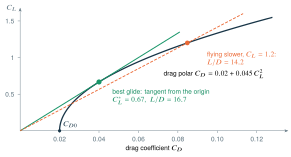
Picture 14.4. The best glide is a tangent. Each point on the drag polar is one way to fly. The slope of the line from the origin to that point is CL/CD, the glide ratio. The steepest such line that still touches the polar is tangent to it, at the point where induced drag KCL2 equals parasite drag CD0.
Best glide. (a) The glide ratio is G(CL)=CD0+KCL2CL for CL>0. Show that G has exactly one critical point, at CL∗=CD0/K, that it is the maximum, and that there induced drag equals parasite drag. (b) With CD0=0.02 and K=0.045, find CL∗ and the best glide ratio. (c) From 1000 m in still air, about how far can the aircraft glide at its best glide ratio? (d) At CL=1.2, flying slower, what is the glide ratio, and how much distance does that cost from 1000 m?
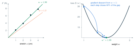
Picture 14.5. Training a one-weight model. Left: the spring data, the least-squares line F=1.99x (aqua, with its four misses drawn) and a worse guess F=1.5x (orange). Right: the loss is a parabola in w, so calculus finds its lowest point exactly; gradient descent (blue) walks down to the same place, closing 60% of the remaining gap at each step.
The smallest machine-learning model. (a) Expand E(w) into a parabola E(w)=αw2−2βw+γ, with α=∑xi2,β=∑xiFi, and γ=∑Fi2. Find its minimizer w∗=β/α and explain why it is the global minimum. (b) For the spring data, find k∗=w∗ and the leftover error E(w∗). (c) Gradient descent updates w←w−ηE′(w). With η=0.01 and w0=1, take two steps. Show that every step multiplies the distance to w∗ by 1−2ηα, and find the range of learning rates η>0 for which the steps converge. (Compare AI01, section 2.6.)
The game engine of M12.21 decides whether a smoke cloud blocks a line of sight with one short function, which both the bots’ perception and the HUD call:
The points of the sight line are start + segment * t for 0≤t≤1:t=0 is the eye and t=1 the target. The std::clamp statement chooses one t and clamps it into [0,1]; the final return asks whether that point lies inside the smoke ball. In the plane of the eye, the target, and the smoke’s centre, glm::dot of two vectors (a1,a2) and (b1,b2) is a1b1+a2b2.
(The closed-interval method in a game engine.) Put the eye at (0,0) and the target at (20,0), in metres, and call the line parameter s (the code’s t), keeping t for time. (a) For smoke centred at (8,3), write the squared distance D2(s) from the point (20s,0) to the centre, minimize it on [0,1], and decide whether a cloud of radius 4.2 m blocks the view. Check that the std::clamp statement computes the same s. (b) Now the smoke is centred at (25,1), beyond the target. Find the s that minimizes D2 with no limits, then the minimum on [0,1]. Is the view blocked? What would the code decide without the clamp, and why would that be wrong? (c) Why may the code (and you) minimize D2 instead of D? (d) By M12.21 the cloud’s radius grows as R(t)=4.2Ec(u), with Ec(u)=3u2−2u3 and u=t/0.8, for 0≤t≤0.8 s. Use the Intermediate Value Theorem and the sign of R′ to show that a sight line passing 3 m from the centre becomes blocked at exactly one moment, between t=0.5 s and t=0.55 s.
Optional small hints
For M14.05, 0<x<6. For M14.06, minimize squared distance instead of its square root. For M14.08, eliminate h with the volume constraint before differentiating.
Compare the first step where your work differs. A corrected answer is not yet an independent success.
M14.01Show solution
Factor the derivative and test intervals
Here f′=3x2−12x+9=3(x−1)(x−3). Its signs are positive before 1, negative between 1 and 3, and positive after 3. Thus the function increases on (−∞,1) and (3,∞) and decreases on (1,3). At 1 it has a local maximum f(1)=4; at 3 a local minimum f(3)=0. These are local, not absolute on R.
Differentiate twice: f′′=12x2−24x=12x(x−2). It is positive on (−∞,0) and (2,∞), negative on (0,2). The graph is continuous and concavity changes at both candidate inputs. Its inflection points are (0,0),(2,−16).
For x4,f′′=12x2≥0 on both sides of zero. The graph stays concave up, so zero is not an inflection input. In fact, it is a local and absolute minimum. A derivative being zero does not by itself describe how its sign behaves nearby.
Let w be each side perpendicular to the river and ℓ the parallel fenced side. The constraint is 2w+ℓ=60, so A=w(60−2w) on 0<w<30. Then A′=60−4w=0 gives w=15,ℓ=30. Since A′′=−4<0 and the endpoint limiting areas vanish, the largest area is 450 m2 with dimensions 15 m by 30 m.
The base dimensions are both 12−2x and height is x. Thus
V=x(12−2x)2,V′=12(x−2)(x−6).
The feasible nondegenerate interval is (0,6). Only x=2 is an interior critical input. V′ is positive before 2 and negative afterward until 6, and limiting endpoint volumes are zero. The maximum is 128 cm3 from a box 8 cm by 8 cm by 2 cm. The zero at 6 describes a collapsed box, not a second useful design.
Squared distance is D(x)=x2+(2x+1)2=5x2+4x+1. Since square root is increasing, minimizing D minimizes distance. Solve D′=10x+4=0 to get x=−2/5, hence y=1/5. The positive second derivative 10 or completed square D=5(x+2/5)2+1/5 proves a global minimum. The point is (−2/5,1/5), at distance 1/5.
Write f=1−1/(x+1), with domain x=−1. The only intercept is (0,0); asymptotes are vertical x=−1 and horizontal y=1. Since f′=1/(x+1)2>0, it increases on each domain interval (−∞,−1) and (−1,∞). It is not increasing across the missing point as a single interval claim. Because f′′=−2/(x+1)3, concavity is up on the left and down on the right. There is no point of the graph at x=−1, so it is not an inflection point.
From πr2h=54π,h=54/r2 with r>0. A closed cylinder has
S(r)=2πr2+2πrh=2πr2+r108π.
Thus S′=4πr−108π/r2=4π(r3−27)/r2. Its unique positive zero is r=3 cm, giving h=6 cm and S=54π cm2. The derivative changes from negative to positive. Also S→∞ as r→0+ or r→∞, so the minimum is global. A very narrow cylinder needs huge height; a very wide one needs huge lids.
Rewrite: f=x4/3−4x1/3. With 34−1=31 and 31−1=−32,
f′(x)=34x1/3−34x−2/3=34x−2/3(x−1).
Critical numbers: x=1, where f′=0, and x=0, where f′ is undefined but f(0)=0 is defined. (The definition agrees that f′(0) does not exist: hf(h)−f(0)=h−2/3(h−4) falls without bound as h→0.) Since x−2/3=1/(x1/3)2>0 for x=0,f′ has the sign of x−1: negative for x<1, on both sides of 0, and positive for x>1. So fdecreases on (−∞,1) and increases on (1,∞), with a local (in fact absolute) minimum f(1)=−3. There is no extremum at 0:f keeps falling through it, along a vertical tangent, since f′→−∞ there.
f′=e−x+x(−e−x)=e−x(1−x) and f′′=−e−x(1−x)+e−x(−1)=e−x(x−2). Because e−x>0, the brackets decide every sign. f increases on (−∞,1) and decreases on (1,∞), with maximum f(1)=1/e≈0.368, absolute by the one-critical-point rule. It is concave down on (−∞,2) and up on (2,∞), with inflection point (2,2/e2)≈(2,0.271).
Derivative on top, then the second derivative test
f′=2xlnx+x2⋅x1=x(2lnx+1). For x>0 it is zero when lnx=−21, at x=e−1/2≈0.607. Next, f′′=2lnx+2+1=2lnx+3, and f′′(e−1/2)=−1+3=2>0, so this is a local minimum, f(e−1/2)=−2e1≈−0.184. Concavity changes where 2lnx+3=0, at x=e−3/2≈0.223: the inflection point is (e−3/2,−2e33)≈(0.223,−0.075), concave down to its left and up to its right.
f′=2sinxcosx=sin(2x), positive on (0,2π) and negative on (2π,π):f rises to its maximum f(2π)=1 and falls back, with minimum 0 at both endpoints. Next, f′′=2cos(2x), positive on (0,4π) and (43π,π) and negative between. So f is concave up, then down, then up, with inflection points (4π,21) and (43π,21).
f′=4x3−12x2=4x2(x−3), so the critical numbers are 0 and 3, and f′′=12x2−24x. At 3:f′′(3)=108−72=36>0, a local minimum, f(3)=−27. At 0:f′′(0)=0, so the second derivative test says nothing. First derivative test: near 0,4x2>0 and x−3<0, so f′<0 on both sides. f keeps decreasing through 0:no extremum there.
f(−x)=−f(x), so the graph is symmetric about the origin. The bottom is never zero, so there is no vertical asymptote, and f→0 as x→±∞: the horizontal asymptote is y=0. Quotient rule: f′=(x2+1)2(x2+1)−x(2x)=(x2+1)21−x2, so f increases on (−1,1) and decreases on (−∞,−1) and (1,∞), with maximum (1,21) and minimum (−1,−21), both absolute. Workbench for f′′, with u=1−x2 and v=(x2+1)−2:u′=−2x and v′=−4x(x2+1)−3, so
Workbench. (1) Minimize the cost C in cents, with base side x and height h in cm. (2) C=2(2x2)+1(4xh). (3) x2h=2000, so h=2000/x2 and C(x)=4x2+x8000 for x>0. (4) With x8000=8000x−1,C′=8x−8000x−2=8x−x28000=x28(x3−1000), zero at x=10. (5) C′<0 before 10 and C′>0 after, so this is the global minimum. The cheapest box is 10 cm×10 cm×20 cm, costing 400+800=1200 cents, $12.00. Because the lids cost double, the best box is twice as tall as it is wide.
The squared distance (M14.06 called it D; here it is D2, so that D is the distance itself) is D2=(x−3)2+(x)2=(x−3)2+x for x≥0. Its derivative 2(x−3)+1 is zero at x=25, its second derivative is 2>0, and it is the only critical point, so it is the global minimum (also D2(0)=9 is larger). The closest point is (25,25)≈(2.5,1.581), with D2=41+25=411, so the distance is 211≈1.658.
If x metres go to the square, its side is x/4; the circle’s circumference is 10−x, so its radius is (10−x)/(2π). Total area on [0,10]:
A(x)=16x2+4π(10−x)2,A′(x)=8x−2π10−x.
Setting A′=0 and multiplying by 8π:πx=4(10−x), so x=π+440≈5.60 m. Since A′′=81+2π1>0, this is the minimum: A=π+425≈3.50 m2, cutting 5.60 m for the square. For the maximum compare the endpoints: A(0)=π25≈7.96 m2 (all circle) and A(10)=6.25 m2 (all square). The largest area comes from not cutting at all: bend the whole wire into a circle, ≈7.96 m2. The circle encloses the most area for its length, so the maximum sits at an endpoint.
R′(θ)=gv2cos(2θ)⋅2, which is zero on (0,2π) only at 2θ=2π, that is θ=4π. The endpoints give R=0, so the maximum is at 45∘, with Rmax=gv2=9.81400≈40.8 m. Half the maximum needs sin(2θ)=21, so 2θ=30∘ or 150∘:θ=15∘ or 75∘. These angles add to 90∘; complementary angles always give equal ranges, because sin(2θ)=sin(180∘−2θ).
For CL>0 it is zero only at CL∗=CD0/K, positive before and negative after, so by the one-critical-point rule this is the maximum. There KCL∗2=CD0: induced drag equals parasite drag, so CD=2CD0 and Gmax=2CD0CL∗=2KCD01.
(b) CL∗=0.02/0.045=4/9=2/3≈0.67 and KCD0=0.0009, so Gmax=2(0.03)1=16.7.
(c) About 16.7×1000 m, roughly 16.7 km.
(d) G(1.2)=0.02+0.045(1.44)1.2=0.08481.2≈14.2, so about 14.2 km: flying slower costs about 2.5 km, because induced drag grows like CL2.
(a) Each term is (Fi−wxi)2=Fi2−2wxiFi+w2xi2, and adding them gives E(w)=αw2−2βw+γ. Then E′(w)=2αw−2β, which is zero at w∗=β/α. Since E′′=2α>0, the parabola opens upward and its vertex is the global minimum; completing the square shows it directly: E=α(w−αβ)2+γ−αβ2.
(b) α=1+4+9+16=30,β=2.1+7.8+18.6+31.2=59.7, and γ=4.41+15.21+38.44+60.84=118.9. So k∗=3059.7=1.99 N/cm, and the leftover error is E(w∗)=γ−αβ2=118.9−118.803=0.097 N2.
(c) E′(w)=60w−119.4. First step: w1=1−0.01(60−119.4)=1.594. Second: w2=1.594−0.01(95.64−119.4)=1.8316. Since 2β=2αw∗, each step gives wn+1−w∗=(wn−w∗)−2ηα(wn−w∗)=(1−2ηα)(wn−w∗); here 1−0.6=0.4, so the gap goes −0.99,−0.396,−0.158, and each step closes 60% of it. The steps converge exactly when ∣1−2ηα∣<1, that is for 0<η<1/α=1/30≈0.033; there is no largest such η, because η=1/30 itself makes the factor −1 and the steps bounce forever. At η=1/60 a single step lands on w∗. AI01’s loss (w−3)2 has α=1, which is why its limit there was η<1.
(a) D2(s)=(20s−8)2+(0−3)2=(20s−8)2+9. Its derivative 40(20s−8) is zero at s=0.4, inside [0,1]; the endpoints give 73 and 153. So the minimum is D2=9,D=3<4.2:blocked. The std::clamp statement computes 202+02(8)(20)+(3)(0)=400160=0.4, the same s, and the clamp leaves it alone.
(b) D2(s)=(20s−25)2+1 has its unlimited minimum at s=1.25, outside [0,1]. On [0,1] its derivative 40(20s−25) is negative, so D2 decreases and the minimum is at the endpoint s=1:D2=26,D≈5.10>4.2,not blocked. Without the clamp the code would use s=1.25, a point 5 m beyond the target, find D=1, and report the target hidden, as if smoke behind a target could hide it. The clamp is the closed-interval method: when the critical point falls outside the interval, an endpoint wins.
(c) D=D2, and the square root is increasing, so D2 and D are smallest at the same s (M14.06). The code takes one square root, inside glm::length, only when it compares with the radius.
(d) R′(t)=0.84.2⋅6u(1−u)>0 for 0<t<0.8, so R increases. R(0.5)=4.2Ec(0.625)≈4.2(0.6836)≈2.871<3 and R(0.55)=4.2Ec(0.6875)≈4.2(0.7681)≈3.226>3.R is continuous, so by the Intermediate Value Theorem R=3 at some t in (0.5,0.55), and because R is increasing, at exactly one. From that moment the sight line is blocked. Module 15’s Newton’s method pins it down: t≈0.518 s.
1. Both endpoints, every interior x where f′(x)=0, and every interior x where f′(x) does not exist. 2. dxd[xe−x]=e−x−xe−x=e−x(1−x). 3. 12x2(x−1)=0, so x=0 or x=1.
Move 4: the chain rule gives dxd4−x2=4−x2−x, so A′(x)=24−x2+2x⋅4−x2−x=4−x22(4−x2)−2x2=4−x28−4x2, zero at x=2; the endpoints give A(0)=A(2)=0. Move 5: A(2)=22⋅2=4, so the best rectangle is 22≈2.83 wide and 2≈1.41 tall, twice as wide as it is tall.
Return to M13.03 and M09.08. Explain the distinct meanings of f=0,f′=0, and f′′=0. Advance when you can derive a feasible objective from an unfamiliar word problem and justify its global optimum, not merely report a critical input.