G04: Probability, information, and credible measurement

Prerequisites and observable goals#

The central question: what population does this number describe?#

A mean without a population and sampling procedure is incomplete. A model accuracy, server error rate, or benchmark speedup is computed from observations, but the desired claim usually concerns different future observations. Identify the unit first: requests, users, independent server restarts, entire workload traces, or machines. A thousand correlated requests from one session are not automatically a thousand independent trials.

Separate three sources of uncertainty. Sampling uncertainty comes from observing a subset of a target population. Measurement error comes from clocks, instrumentation, rounding, and collection mistakes. Modeling error comes from assumptions such as independent arrivals or a workload that fails to represent deployment. More repeated runs can reduce some sampling uncertainty without repairing an unrealistic workload.

Conditional probability as a changed denominator#

For events $A,B$ with $P(B)>0$, $P(A\mid B)=P(A\cap B)/P(B)$. The condition restricts the sample space. Multiplication gives $P(A\cap B)=P(B\mid A)P(A)$, and partitioning by $A$ and its complement yields

A detector’s sensitivity cannot be read as the reliability of a flag without prevalence. For a rare fault with prevalence .02, sensitivity .8, and false-positive probability .1, the joint true-positive probability is $.016$ and false-positive probability $.098$. Among flags, the true fraction is $.016/.114=8/57\approx.1404$. Replacing a probability tree with 10,000 cases often makes the denominator visible.

Independence means $P(A\cap B)=P(A)P(B)$. Conditional independence given $C$ is a separate statement. Two measurements can be correlated because they share a hidden workload class, even if independent after conditioning on that class. Splitting data by row while duplicating that shared class across training and test can exploit a dependency rather than demonstrate generalization.

Expectation, variance, and a concentration calculation#

For independent identically distributed Bernoulli variables $X_i$ with success probability $p$, the sample proportion $\hat p=n^{-1}\sum_iX_i$ has expectation $p$ and variance $p(1-p)/n$. Linearity of expectation does not require independence; removing covariance terms from the variance does. For dependent variables,

Positive dependence can make the naive independent standard error too small.

For independent variables bounded in $[0,1]$, Hoeffding’s inequality gives

To make the upper bound at most $\delta$, solve $2e^{-2n\epsilon^2}\le\delta$: take logarithms, rearrange, and obtain

For $\epsilon=.1,\delta=.05$, this requires $n\ge184.44\ldots$, hence 185 observations. This is a distribution-free bound under independence and boundedness, not a claim that 185 arbitrary correlated records certify every prediction. The inequality is stated here; the calculation using it is derived. A deeper probability course should prove the exponential-moment bound underlying it.

A proportion interval that behaves near the endpoints#

The simple symmetric approximation $\hat p\pm1.96\sqrt{\hat p(1-\hat p)/n}$ degenerates to zero width when all trials agree. The Wilson score interval instead inverts a standardized discrepancy using the hypothesized $p$ in its variance. With critical value $z$, its center and half-width are

For 18 successes in 20 trials and $z=1.96$, the interval is approximately $[.6990,.9721]$. The confidence level is a property of a repeated-sampling procedure under its model; it is not a frequentist probability that a fixed unknown parameter lies in the already computed interval. For clustered records, a binomial interval may not match the sampling design. Report the count and denominator with the interval, not only a rounded percentage.

Paired comparisons and bootstrap logic#

Suppose the same workload trace is run on old and new implementations. Define $d_i=t_{{\rm new},i}-t_{{\rm old},i}$. Negative values favor the new version. Pairing removes some variation caused by easy versus difficult traces. Resampling pairs means resampling the differences $d_i$, not independently resampling the two timing columns. The lab computes bootstrap means from samples of those differences and takes percentile endpoints.

This percentile bootstrap is an exploratory interval, not a universal guarantee. With very few pairs, severe dependence, time trends, or biased workload selection, it can mislead. A paired $t$ method or an appropriate hierarchical/block design may be preferable under its own assumptions. Establish the experimental unit before selecting a resampling scheme.

Worked example: old times $(10,20,30)$ and new times $(8,18,28)$ give differences $(-2,-2,-2)$. Every resample has mean $-2$, so the bootstrap interval collapses to $[-2,-2]$. That does not establish that every future workload saves exactly two units. It shows that these three paired observations contain no observed variation in their differences; the uncertainty model has no information about unsampled behavior.

Information measures and their limits#

For a discrete probability vector $p$, entropy in bits is $H(p)=-\sum_i p_i\log_2p_i$, with the continuous extension $0\log0=0$. A certain event has entropy zero. Two equally likely outcomes have one bit; probabilities $(1/2,1/4,1/4)$ give $1/2+1/2+1/2=1.5$ bits. This quantifies distributional uncertainty, not semantic importance or human intelligence.

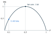
Cross-entropy under a proposed distribution $q$ is $H(p,q)=-\sum_i p_i\log q_i$. With matching logarithm bases, $H(p,q)=H(p)+D_{\rm KL}(p\Vert q)$, where $D_{\rm KL}=\sum_i p_i\log(p_i/q_i)\ge0$ when properly defined. If $p_i>0$ and $q_i=0$, the term is infinite. KL is not a symmetric distance. In binary classification, empirical cross-entropy rewards assigning probability to the observed class; it does not by itself prove calibration under distribution shift.

Independent practice#

F foundation C standard course work T transfer S optional stretch L runnable lab or project. Attempt the complete set before opening its solutions.

Smallest useful hints#

For .02, round upward only after solving the logarithmic inequality. For .03, set $\hat p=0$ in both center and half-width. For .04, inspect the distribution of differences, not merely the two marginal distributions.

Complete solutions: G04#

Compare the first step where your work differs. A corrected answer is not yet an independent success.

Open every solution

"""G04: explicit statistical procedures; validity still needs a sampling model."""
import math
import random


def wilson(successes, trials, z=1.96):
    if type(trials) is not int or type(successes) is not int or not 0 <= successes <= trials or trials < 1:
        raise ValueError("integer counts with 0 <= successes <= trials required")
    if not math.isfinite(z) or z <= 0:
        raise ValueError("finite positive critical value required")
    p = successes / trials
    denominator = 1 + z*z/trials
    center = (p + z*z/(2*trials)) / denominator
    half = z*math.sqrt(p*(1-p)/trials + z*z/(4*trials*trials)) / denominator
    return max(0., center-half), min(1., center+half)


def entropy(probabilities):
    p = list(probabilities)
    if not p or any(not math.isfinite(x) or x < 0 or x > 1 for x in p):
        raise ValueError("nonempty finite probability vector required")
    if not math.isclose(math.fsum(p), 1., rel_tol=0., abs_tol=1e-12):
        raise ValueError("probabilities must sum to one")
    return -math.fsum(x*math.log2(x) for x in p if x > 0)


def quantile(values, probability):
    values = sorted(values)
    if not values or not math.isfinite(probability) or not 0 <= probability <= 1:
        raise ValueError("nonempty data and probability in [0,1] required")
    if any(not math.isfinite(x) for x in values):
        raise ValueError("finite observations required")
    position = (len(values)-1)*probability
    lo = math.floor(position)
    hi = min(lo+1, len(values)-1)
    fraction = position-lo
    return (1-fraction)*values[lo]+fraction*values[hi]


def paired_bootstrap(old, new, repeats=2000, seed=21, confidence=.95):
    if len(old) != len(new) or not 2 <= len(old) <= 10000:
        raise ValueError("2..10000 matched pairs required")
    if type(repeats) is not int or not 100 <= repeats <= 10000:
        raise ValueError("100..10000 resamples required")
    if not math.isfinite(confidence) or not 0 < confidence < 1:
        raise ValueError("confidence must lie in (0,1)")
    if any(not math.isfinite(v) for v in [*old, *new]):
        raise ValueError("finite measurements required")
    differences = [b-a for a,b in zip(old,new)]
    if any(not math.isfinite(d) for d in differences):
        raise ValueError("difference overflow")
    rng = random.Random(seed)
    n = len(differences)
    means = [math.fsum(rng.choice(differences) for _ in range(n))/n
             for _ in range(repeats)]
    tail = (1-confidence)/2
    return {"mean_difference": math.fsum(differences)/n,
            "interval": (quantile(means,tail),quantile(means,1-tail)),
            "seed":seed,"pairs":n,"resamples":repeats}


if __name__ == "__main__":
    print("Wilson:",wilson(18,20))
    print("Entropy:",entropy([.5,.25,.25]))
    print(paired_bootstrap([10,20,30],[8,18,28]))

Readiness and next depth#

You should be able to name the sampling unit and write the conditional denominator before calculating. Review foundation A03–A04 when those choices are unclear. Continue with concentration proofs, stochastic processes, hierarchical models, and experimental design; do not claim the elementary bootstrap lab covers those areas. Connect the interval exercise to G16’s research review and G15’s group-aware splitting.