Module 25: Introductory differential equations and dynamical models

8 exercises, each with a complete solution. 1 figure. 1 note from the engine.

On this page

A. Prerequisites and observable goals
B. The central idea: the unknown is a function
C. Three tools with different purposes
D. Why separation and integrating factors work
E. A modeling and solving sequence
F. Worked examples
Computing bridge: The equation, the stepper, and the experiment are different objects
G. Independent practice
H. Complete solutions: Module 25
I. Retention and readiness

A. Prerequisites and observable goals#

Before

Antiderivatives, chain and product rules, exponentials, and initial values.

After

Recognize separable and first-order linear equations, preserve equilibrium solutions, verify an initial-value solution, and interpret Euler approximations.

B. The central idea: the unknown is a function#

A differential equation relates an unknown function to its derivatives. A solution must satisfy that relationship throughout an interval, not merely at one input. An initial condition selects a particular trajectory when suitable existence and uniqueness conditions hold. This module is a selected introduction, not a full differential-equations course. Linear equations and autonomous phase-line analysis may be optional in a particular calculus syllabus.

A differential equation is a field of slopes. For

y'=1-\tfrac y2

the short grey marks show the slope a solution must have at each point. Three solutions are drawn, starting at

0

1

, and

3.8

; each follows the marks, and all approach the equilibrium

y=2

, where the slope is zero.

C. Three tools with different purposes#

A separable equation has the form $y'=g(t)h(y)$ . Where $h(y)\ne0$ , integration of $y'/h(y)=g(t)$ leads to $\int\dd y/h(y)=\int g(t)\dd t$ . Constant solutions satisfying $h(y)=0$ must be checked separately because division removes them.

A first-order linear equation has form $y'+p(t)y=q(t)$ . On an interval where $p,q$ are continuous, an integrating factor

\mu(t)=e^{\int p(t)\dd t}

turns the left side into $(\mu y)'$ , so $\mu y=\int\mu q\dd t+C$ . A coefficient singularity may limit the solution interval.

For $y'=f(t,y)$ , the Euler method advances a tangent approximation:

t_{n+1}=t_n+h,\qquad y_{n+1}=y_n+h f(t_n,y_n).

It generally produces approximate values, not an exact solution. Smaller $h$ need not rescue a bad model or a mistaken update order. Standard methods: [O2ODE].

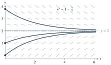
For an autonomous equation $y'=h(y)$ , zeros of $h$ are equilibria, and its sign gives increasing or decreasing motion between them. Local uniqueness, for example when $f$ and $\partial f/\partial y$ are continuous near initial data, prevents distinct solution curves from crossing there. Without uniqueness hypotheses, such a claim is unsafe.

D. Why separation and integrating factors work#

Separation is the chain rule in reverse: if $H'(y)=1/h(y)$ , then $\dd H(y(t))/\dd t=y'/h(y)=g(t)$ . The differential shorthand does not require treating derivatives as ordinary fractions without justification.

For a linear equation, choose $\mu$ so that $\mu'=p\mu$ . Then the product rule gives $(\mu y)'=\mu y'+p\mu y=\mu q$ . The exponential formula solves precisely this requirement. It is constructed to create an exact product derivative, not guessed from an unrelated pattern.

E. A modeling and solving sequence#

State the dependent quantity and time units. Build a rate balance: accumulation equals input rate minus output rate. Identify the equation type, solve on a domain interval, restore any equilibrium solutions lost by division, apply initial data, and substitute the resulting function back into the original equation. For a physical model, also check nonnegativity and whether a finite-time singularity signals a model limit.

F. Worked examples#

Exponential decay. If $y'=-ky$ with $k>0$ , separation for nonzero $y$ gives $\ln|y|=-kt+C$ , hence $y=Ae^{-kt}$ . The equilibrium $y=0$ is included by allowing $A=0$ . With $y(0)=y_0$ , $A=y_0$ . The half-life satisfies $e^{-kT}=1/2$ , so $T=\ln2/k$ .

A linear forced model. For $y'+2y=6$ , $y(0)=1$ , take $\mu=e^{2t}$ . Integrating $(e^{2t}y)'=6e^{2t}$ yields $y=3+Ce^{-2t}$ . The initial condition gives $C=-2$ , so $y=3-2e^{-2t}$ . Substitution verifies both the equation and the starting value; the long-term value $3$ balances forcing against removal.

A phase-line interpretation. For $y'=y(2-y)$ , the equilibria are $0,2$ . Rates are negative below $0$ , positive between $0,2$ , and negative above $2$ . Positive starting populations move toward $2$ , while $0$ is unstable to positive perturbations. The arrows describe the differential equation’s behavior; they do not specify all physical validity assumptions of a population model.

Computing bridge: The equation, the stepper, and the experiment are different objects#

For $y'=-y$ , $y(0)=1$ , the model has exact solution $e^{-t}$ . Euler produces $y_{n+1}=(1-h)y_n$ , a discrete approximation. It decays stably for $0<h<2$ , but for $1<h<2$ it alternates sign even though the exact solution stays positive. A06 and T04 use this distinction to show why stability, accuracy, and physical plausibility must be checked separately. A changing frame time is a numerical-method decision, not only an animation convenience.

From the engine: Fate EngineA health bar that solves a differential equation

When a target loses health, Fate Engine does not snap the bar to the new value. The displayed value $y$ chases the true value $T$ at a rate proportional to the gap: $y' = -k\,(y - T)$ . This module’s first-order linear equation has the solution $y(t + \Delta t) = T + (y(t) - T)\,e^{-k\Delta t}$ , and the code is that solution with $\alpha = 1 - e^{-k\Delta t}$ .

Fate Engine: the target frame's health barC++

float targetFrameSmoothedRatio(
    float displayedRatio,
    float targetRatio,
    float deltaTime,
    float response) {
    const float current = std::isfinite(displayedRatio)
        ? std::clamp(displayedRatio, 0.0f, 1.0f)
        : 0.0f;
    const float target = std::isfinite(targetRatio)
        ? std::clamp(targetRatio, 0.0f, 1.0f)
        : 0.0f;
    if (!std::isfinite(deltaTime) || deltaTime <= 0.0f) return current;
    if (!std::isfinite(response) || response <= 0.0f) return target;

    const float alpha = 1.0f - std::exp(-response * deltaTime);
    const float smoothed = current + (target - current) * alpha;
    return std::abs(target - smoothed) < 0.0005f
        ? target
        : std::clamp(smoothed, 0.0f, 1.0f);
}

Because each step is the exact solution, the bar moves the same way at any frame rate. With $k = 12$ per second, one frame at 30 Hz closes $1 - e^{-0.4} = 32.97$ percent of the gap, and four frames at 120 Hz close exactly the same amount. The shortcut $\alpha = k\,\Delta t$ , which is Euler’s method, closes 40 percent at 30 Hz but 34.39 percent over four frames at 120 Hz, so the animation would depend on the machine. The gap halves every $\ln 2/k \approx 57.8$ ms.

G. Independent practice#

F foundation C standard course work T transfer S optional stretch L runnable lab or project. Attempt the complete set before opening its solutions.

M25.01FSolution

Solve $y'=3y$ , $y(0)=2$ , and verify the result.

M25.02CSolution

Solve $y'=2t(1+y^2)$ , $y(0)=0$ , on the maximal interval around zero where the formula is finite.

M25.03TSolution

Solve $y'=y^2$ , $y(0)=1$ . State its maximal interval containing zero and identify an equilibrium lost by separation.

M25.04CSolution

Solve $y'+y=e^{2t}$ , $y(0)=0$ , using an integrating factor.

M25.05TSolution

A $100$ L well-mixed tank initially contains $20$ kg of salt. Pure water enters at $5$ L/min and solution leaves at $5$ L/min. Find the salt amount and its half-life under this model.

M25.06CSolution

Use Euler’s method with $h=1/2$ for two steps to approximate $y(1)$ when $y'=t+y$ , $y(0)=1$ .

M25.07TSolution

For $y'=y(3-y)$ , find equilibria and describe the direction of motion for $0<y<3$ and $y>3$ . Classify the stability of the positive equilibrium.

M25.08SSolution

The equation $y'=2\sqrt{|y|}$ has initial condition $y(0)=0$ . Show that both $y\equiv0$ and, for each $c\ge0$ , the function $y(t)=0$ for $t\le c$ and $y(t)=(t-c)^2$ for $t>c$ solve the initial-value problem. Explain the uniqueness issue.

Optional small hints

For M25.02, integrate to an arctangent before solving for $y$ . For M25.05, outflow concentration is current amount divided by current volume. For M25.08, check the derivative at the joining time, not just on either side.

H. Complete solutions: Module 25#

Compare the first step where your work differs. A corrected answer is not yet an independent success.

M25.01Show solution

An exponential trajectory selected by initial data

Separation or recognition gives $y=Ce^{3t}$ . At $t=0$ , $C=2$ , so $\boxed{y=2e^{3t}}$ for all real $t$ . Differentiating gives $y'=6e^{3t}=3y$ , and $y(0)=2$ . Both the differential equation and the initial condition are verified.

Back to M25.01

M25.02Show solution

An implicit antiderivative exposes the solution’s interval

Since $1+y^2>0$ , separation gives $\arctan y=t^2+C$ . Initial data imply $C=0$ , so $y=\tan(t^2)$ near zero. The first poles occur at $t^2=\pi/2$ , giving maximal interval $\boxed{(-\sqrt{\pi/2},\sqrt{\pi/2})}$ . Its derivative is $2t\sec^2(t^2)=2t(1+y^2)$ , as required. The solution cannot be extended through a pole as a finite differentiable real function.

Back to M25.02

M25.03Show solution

Finite-time blow-up and a discarded equilibrium

For nonzero $y$ , integrate $y^{-2}\dd y=\dd t$ to obtain $-1/y=t+C$ . The initial value gives $C=-1$ , hence $\boxed{y=1/(1-t)}$ . The maximal connected interval containing zero is $\boxed{(-\infty,1)}$ . Its derivative is $(1-t)^{-2}=y^2$ . The constant function $y=0$ is also a solution of the differential equation, although it does not satisfy this particular initial condition and was excluded by division.

Back to M25.03

M25.04Show solution

Build an exact product derivative

The integrating factor is $e^t$ . Multiplying gives $(e^ty)'=e^{3t}$ . Integration yields $e^ty=e^{3t}/3+C$ , so $y=e^{2t}/3+Ce^{-t}$ . The initial condition gives $C=-1/3$ , hence $\boxed{y=(e^{2t}-e^{-t})/3}$ . Differentiating and adding $y$ cancels the $e^{-t}$ terms and produces $e^{2t}$ .

Back to M25.04

M25.05Show solution

A concentration is not an amount

Let $S(t)$ be salt mass in kg. The volume stays $100$ L. Salt enters at zero rate and leaves at $5(S/100)=S/20$ kg/min. Thus $S'=-S/20$ , $S(0)=20$ , giving $\boxed{S(t)=20e^{-t/20}}$ for physical times $t\ge0$ . The half-life solves $e^{-t/20}=1/2$ , so $\boxed{20\ln2\text{ min}}$ . Nonnegative mass decays toward zero, consistent with flushing by pure water.

Back to M25.05

M25.06Show solution

Use the old time and old value at each step

At $(t_0,y_0)=(0,1)$ , the slope is $1$ , so $y_1=1+(1/2)(1)=3/2$ at $t_1=1/2$ . The next slope is $1/2+3/2=2$ , giving $y_2=3/2+(1/2)(2)=\boxed{5/2}$ at $t_2=1$ . This is approximate. The exact solution $y=2e^t-t-1$ gives $y(1)=2e-2\approx3.43656$ , illustrating substantial coarse-step error.

Back to M25.06

M25.07Show solution

Read the sign of the rate, not the height

The equilibria satisfy $y(3-y)=0$ , so they are $0,3$ . For $0<y<3$ , both factors are positive and the solution increases. For $y>3$ , the second factor is negative and the solution decreases. Nearby values on both sides move toward $3$ , so the positive equilibrium is stable and attracting. Smoothness of the polynomial rate supplies local uniqueness, preventing a trajectory from crossing the equilibrium and continuing through it.

Back to M25.07

M25.08Show solution

Continuous right sides need not guarantee uniqueness

For $t<c$ , the proposed solution and derivative are zero, matching $2\sqrt{|y|}=0$ . For $t>c$ , $y' =2(t-c)$ and $2\sqrt{(t-c)^2}=2(t-c)$ because $t-c>0$ . At $t=c$ , both one-sided derivatives are zero, so the function is differentiable there and satisfies the equation. Since $c\ge0$ , the initial value is zero. These are distinct solutions, including arbitrary waiting times. The right side is continuous but is not locally Lipschitz in $y$ at zero; its $y$ derivative does not provide the usual continuous-derivative uniqueness hypothesis there.

Back to M25.08

I. Retention and readiness#

Revisit M20.01, M03.07, and M12.06. Explain why a proposed solution is checked by both differentiation and initial substitution. Use Mixed Review R2 next; count a method selected only after seeing a hint as assisted, not independent.