T03: Machine learning, gradients, evaluation, and attention

A. Prerequisites and observable goals#

Level: Advanced-entry track. Small models and synthetic data, not frontier-model development or a complete ML research education.

B. The central question: what is learned, and how would you know it generalizes?#

A supervised model maps features $x$ to a prediction using parameters learned from labeled examples. An objective assigns a cost to predictions; an optimizer changes parameters to reduce training cost. A low training cost is not evidence by itself that the model works on new data. The training distribution, label quality, split design, and evaluation metric all affect the interpretation.

Start with linear regression: $\hat y=w^Tx+b$. Squared-error minimization connects to A02 least squares, while gradient descent provides an iterative route. For binary classification, a linear score $z=w^Tx$ can be mapped to a number between zero and one by the logistic sigmoid

We include an intercept by making the first feature $x_0=1$, so $w_0$ plays the role of $b$. A prediction probability is a model output under assumptions, not an established fact about an individual. A threshold converts it into a decision, and the costs of false positives and false negatives can justify thresholds other than $0.5$.

The companion uses ordinary Python and small dense lists so every operation is visible. This is not a performance-oriented tensor library. Frameworks become useful after the learner can explain shapes, objectives, gradients, and data boundaries independently.

C. Derive the objective and gradient#

For label $y\in\{0,1\}$ and probability $p=\sigma(z)$, binary cross-entropy is

An equivalent form is $\log(1+e^z)-yz$. To avoid overflow for large positive $z$, evaluate it as

This is the same real-valued function, evaluated with a more suitable numerical expression. The stable sigmoid similarly uses $e^{-z}$ when $z\ge0$ and $e^z/(1+e^z)$ when $z<0$.

Differentiate the softplus form: $\partial\ell/\partial z=\sigma(z)-y$. Since $z=\sum_jw_jx_j$, the chain rule gives

For $n$ examples and $L_2$ regularization excluding the intercept,

for $j\ge1$, with no regularization term for $j=0$. Regularization penalizes large coefficients under this representation; feature scaling changes its effect, so preprocessing is part of the model definition.

A gradient step is $w\gets w-\alpha\nabla J(w)$. The minus sign moves locally against the direction of steepest increase. A step size that is too large can overshoot or diverge; reducing loss on one step is not a proof of convergence for all objectives. Logistic regression with this convex objective has a much simpler optimization landscape than a general neural network, but finite data, conditioning, and stopping still matter.

D. Backpropagation is the chain rule over a computation graph#

Our tiny network has two input features and one hidden unit:

Let $g=\sigma(z)-y$. Then

Multiplying the last expression by $x_0$, $x_1$, or $1$ yields derivatives with respect to $w_0,w_1,b$. Backpropagation reuses intermediate values instead of symbolically expanding the entire composition separately for each parameter.

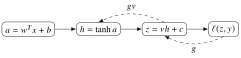
Solid arrows are forward dependencies; dashed arrows illustrate derivatives propagated backward. The stored activation $h$ supplies the local derivative $1-h^2$. This is an exact chain-rule derivation for the mathematical network, evaluated approximately in floating point.

A finite-difference gradient check compares each analytic component with

Use several moderate parameter vectors, an appropriate small $\varepsilon$, and absolute/relative tolerances. Too-small steps amplify roundoff; too-large steps increase truncation error. Gradient agreement is strong debugging evidence for those cases, not a proof that every training configuration is correct. Automatic differentiation computes derivatives through program operations; it is distinct from both finite differences and symbolic algebra.

E. Evaluation boundaries are part of the algorithm#

Training data determines parameters. Validation data supports model and hyperparameter choices. A held-out test set estimates performance after choices are fixed. Repeatedly inspecting test results and adjusting the model turns the test set into another validation set. Standardization means and scales must be fit on training data only and then reused unchanged for validation and test examples. Fitting preprocessing on the whole dataset leaks information even without directly using test labels.

Split design must match the future use case. Random row splitting can leak near-duplicate users, sessions, or adjacent time points across sets. A future-time evaluation may require a chronological split; a new-user task may require grouping by user. The synthetic lab generates independent examples under one fixed mechanism, so simple disjoint index ranges are adequate for its limited demonstration. Real data requires a more careful independence argument.

Accuracy is $(TP+TN)/N$, precision is $TP/(TP+FP)$ when defined, and recall is $TP/(TP+FN)$ when defined. A classifier predicting the majority class can have high accuracy while missing every rare positive. Evaluate relevant slices, threshold tradeoffs, calibration, label noise, and uncertainty. Correlation between a feature and outcome does not establish that changing the feature would cause the outcome to change.

The reference run generated 180 synthetic examples with seed 20260905, split into 108 training, 36 validation, and 36 test examples. With fixed hyperparameters, it recorded validation loss $0.1858900$ and test accuracy $32/36\approx0.8889$. This is one small synthetic experiment, not a generalization claim for real game users or a benchmark against commercial AI. Four errors remain and should be examined rather than hidden by the average.

F. Embeddings and a bounded introduction to attention#

An embedding table maps discrete token identifiers to learned vectors. A lookup selects rows; training changes those vectors through the objective. Similarity of embeddings depends on how they were trained and evaluated, not on a guarantee that every direction has a human-interpretable meaning.

For query matrix $Q\in\R^{n_q\times d}$, key matrix $K\in\R^{n_k\times d}$, and value matrix $V\in\R^{n_k\times d_v}$, scaled dot-product attention is

where softmax is applied across each query’s key scores. Each row produces nonnegative weights summing to one and forms a weighted sum of value rows. Subtracting a row’s maximum score before exponentiation improves numerical stability without changing the exact softmax. The original Transformer paper supplies this operation and the surrounding encoder/decoder architecture; the companion implements only this small attention calculation. [ATTN]

For one zero query, all finite dot products are zero, so two keys receive equal weights and the output is the average of their value vectors. This does not require the keys themselves to be equal. A causal mask in a sequence model prevents a position from using future positions when predicting the next token. Positional information, multiple heads, residual paths, normalization, feed-forward layers, an output objective, and training are additional mechanisms; attention alone is not a language model.

A productive first paper-reading pass identifies the problem, assumptions, central equation, input/output shapes, and evaluation design. On a second pass, reproduce a small operation and check a claim against a controlled example. On a third, examine ablations, limitations, and alternative explanations. Reproducing this attention equation is an entry exercise, not a reproduction of the paper’s full training experiments.

G. Independent practice#

F foundation C standard course work T transfer S optional stretch L runnable lab or project. Attempt the complete set before opening its solutions.

H. Complete solutions: T03#

Compare the first step where your work differs. A corrected answer is not yet an independent success.

Open every solution

"""T03.05: logistic training, analytic gradients, tiny backprop, attention."""
import math
import random

def sigmoid(z):
    if z >= 0:
        return 1 / (1 + math.exp(-z))
    ez = math.exp(z)
    return ez / (1 + ez)

def loss_grad(weights, rows, labels, l2=0.0):
    if not rows or len(rows) != len(labels) or not weights:
        raise ValueError("nonempty compatible dataset required")
    if any(len(row) != len(weights) for row in rows):
        raise ValueError("feature/weight shape mismatch")
    if not math.isfinite(l2) or l2 < 0 or any(y not in (0, 1) for y in labels):
        raise ValueError("binary labels and nonnegative regularization required")
    if any(not math.isfinite(x) for row in rows for x in row) or any(
            not math.isfinite(w) for w in weights):
        raise ValueError("finite data required")
    grad = [0.0] * len(weights)
    losses = []
    for x, y in zip(rows, labels):
        z = math.fsum(w * v for w, v in zip(weights, x))
        if not math.isfinite(z): raise ArithmeticError("nonfinite logit")
        losses.append(max(z, 0) - y*z + math.log1p(math.exp(-abs(z))))
        error = sigmoid(z) - y
        for j, v in enumerate(x): grad[j] += error * v / len(rows)
    loss = math.fsum(losses) / len(rows)
    for j in range(1, len(weights)):  # do not regularize intercept
        loss += 0.5 * l2 * weights[j]**2
        grad[j] += l2 * weights[j]
    return loss, grad

def fit(rows, labels, epochs=400, rate=0.2, l2=0.01):
    if type(epochs) is not int or epochs <= 0 or not math.isfinite(rate) or rate <= 0:
        raise ValueError("positive training budget and rate required")
    if not rows: raise ValueError("empty dataset")
    weights = [0.0] * len(rows[0])
    for _ in range(epochs):
        _, grad = loss_grad(weights, rows, labels, l2)
        weights = [w - rate*g for w, g in zip(weights, grad)]
    return weights

def tiny_network(params, x, y):
    """One tanh hidden unit: params=(w0,w1,b,v,c); returns BCE and gradient."""
    if len(params) != 5 or len(x) != 2 or y not in (0, 1):
        raise ValueError("five parameters, two features, binary target required")
    if any(not math.isfinite(a) for a in list(params) + list(x)):
        raise ValueError("finite parameters and features required")
    w0, w1, b, v, c = params
    h = math.tanh(w0*x[0] + w1*x[1] + b)
    z = v*h + c
    g = sigmoid(z) - y
    inner = g*v*(1-h*h)
    loss = max(z, 0) - y*z + math.log1p(math.exp(-abs(z)))
    return loss, [inner*x[0], inner*x[1], inner, g*h, g]

def attention(q, k, v):
    if not q or not k or len(k) != len(v) or not q[0] or not v[0]:
        raise ValueError("nonempty compatible Q,K,V required")
    d, dv = len(q[0]), len(v[0])
    if any(len(row) != d for row in q + k) or any(len(row) != dv for row in v):
        raise ValueError("inconsistent attention dimensions")
    if any(not math.isfinite(x) for row in q+k+v for x in row):
        raise ValueError("finite attention inputs required")
    out = []
    for query in q:
        scores = [math.fsum(a*b for a, b in zip(query, key))/math.sqrt(d)
                  for key in k]
        if any(not math.isfinite(s) for s in scores):
            raise ArithmeticError("attention score overflow")
        exps = [math.exp(s - max(scores)) for s in scores]
        weights = [e/math.fsum(exps) for e in exps]
        out.append([math.fsum(w*value[j] for w, value in zip(weights, v))
                    for j in range(dv)])
    return out

def experiment(seed=20260905):
    rng = random.Random(seed)
    raw, labels = [], []
    for _ in range(180):
        x = [rng.uniform(-2, 2), rng.uniform(-2, 2)]
        raw.append(x)
        labels.append(int(x[0] + 0.5*x[1] + rng.gauss(0, 0.4) > 0))
    # Disjoint fixed index ranges; preprocessing is fitted on training only.
    train, validation, test = range(108), range(108, 144), range(144, 180)
    means = [math.fsum(raw[i][j] for i in train)/len(train) for j in range(2)]
    scales = [math.sqrt(math.fsum((raw[i][j]-means[j])**2 for i in train)
                        /len(train)) for j in range(2)]
    rows = [[1.] + [(x[j]-means[j])/scales[j] for j in range(2)] for x in raw]
    w = fit([rows[i] for i in train], [labels[i] for i in train])
    val_loss = loss_grad(w, [rows[i] for i in validation],
                         [labels[i] for i in validation])[0]
    correct = sum((sigmoid(math.fsum(a*b for a, b in zip(w, rows[i]))) >= .5)
                  == bool(labels[i]) for i in test)
    return {"weights": w, "validation_loss": val_loss,
            "test_accuracy": correct/len(test), "test_count": len(test),
            "split_sizes": [len(train), len(validation), len(test)], "seed": seed}

if __name__ == "__main__":
    print(experiment())

I. Retention and readiness#

Retrieve M10 chain rules, multivariable gradients, A02 least squares, and A04 evaluation uncertainty. Readiness requires deriving a gradient, diagnosing leakage, and explaining errors on fresh examples without relying on a framework to hide the math. ML engineering adds data pipelines and deployment; AI research adds deeper statistics, optimization, literature analysis, and novel experimental questions; infrastructure engineering emphasizes reliable compute and storage. These paths overlap but are not interchangeable.