F01: Feedback control: derivatives that fly drones and steer cars

A. Prerequisites and observable goals#

Level: Frontier track, reachable in Calculus I. Simulated vehicles only. Real aircraft and vehicles add hardware, safety, and regulatory work that this chapter does not replace.

B. The central idea: measure, compare, push, repeat#

Every autopilot is a loop. A drone holding altitude, a car staying in its lane, a rocket landing on a pad: each one measures where it is, compares that with where it should be, and pushes a little in the right direction. Then it does it again, hundreds of times a second.

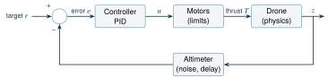
The loop in every autopilot. Each box has a job, and each arrow is a signal with units.

Four words carry the whole subject. The plant is the thing being controlled (the drone and its physics). The setpoint or target $r$ is where you want it. The error is $e=r-z$. The controller turns error into a command. Everything else in this chapter is about choosing that command well, and about the ways a real loop fights back: motor limits, noisy sensors, and actuators that cannot move instantly.

C. The plant: a drone that wants to fall#

Put a drone of mass $m$ on a vertical line. Its altitude is $z(t)$, its vertical velocity is $z'(t)$, and its acceleration is $z''(t)$, exactly the position, velocity, and acceleration chain from Module 12. Three forces act on it: motor thrust $T$ upward, weight $mg$ downward, and air drag $cz'$ opposing motion. Newton’s second law gives the plant model

Read it like a mechanic. If thrust equals weight and the drone is still, then $z''=0$ and nothing changes: that is a hover. More thrust accelerates it up; less lets gravity win. The controller’s only lever is $T$, and the motors can supply only $0\le T\le T_{\max}$. They cannot pull the drone down.

The lab uses $m=1.5$ kg, $c=0.3$ N$\cdot$s/m, $g=9.81$ m/s$^2$, and $T_{\max}=2mg\approx29.43$ N. A computer cannot solve the model with calculus symbols, so it steps time forward in ticks of $\Delta t=0.01$ s:

This is the derivative used backwards: a rate times a small time step gives a small change. It is the same update a game engine’s fixed-step physics performs every frame.

D. Proportional control and the error that never goes away#

The simplest controller pushes in proportion to the error: $T=K_Pe$. Try it and the drone climbs, then stops short of the target and stays there (orange curve below). Before running anything, you can predict exactly how short.

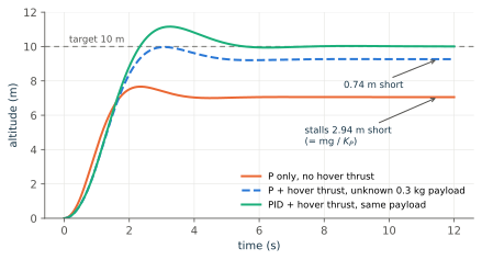
Raising $K_P$ shrinks the gap, but a gain large enough for a 5 cm error (about 294 N/m) asks for 294 N of thrust per metre of error. The motors saturate, and sensor noise gets multiplied by the same huge number. Better tools exist.

E. Three fixes, one idea each#

Feedforward: add what you already know. You know hovering needs about $mg$ of thrust, so add it before feedback does anything: $T=mg_{\text{est}}+K_Pe$. With a perfect mass estimate, the steady-state error becomes zero (dashed blue, until a 0.3 kg payload appears). Now the leftover weight $0.3g$ must come from $K_Pe$, giving $e=0.3(9.81)/4\approx0.74$ m.

Integral: remember the past. Add $K_I\int_0^t e\,\dd\tau$. While any error remains, the integral keeps growing, and so does the thrust it adds. The only resting state is $e=0$, which is why the aqua curve reaches the target even though nobody told the controller about the payload. This is an accumulation, the idea behind every integral in Module 16.

Derivative: damp the motion. Add $-K_D\,z'$, a push against vertical velocity. It acts like a shock absorber. It resists fast motion without caring where the drone is, which cuts overshoot. The complete controller is

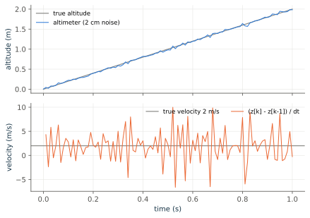
The catch: derivatives amplify noise. A computer estimates $z'$ from samples with a backward difference, $(z_k-z_{k-1})/\Delta t$. That is the secant slope from Module 08. Suppose the altimeter adds independent noise of standard deviation $\sigma$ to each reading. The difference of two readings has noise $\sqrt{2}\,\sigma$, and dividing by a tiny $\Delta t$ magnifies it:

F. Motors have limits: saturation and windup#

Command a 50 m climb and the controller asks for more thrust than the motors have. The output is clipped at $T_{\max}$, the saturation limit, but the integral does not know that. It keeps accumulating error through the whole climb, and when the drone finally reaches 50 m, that stored integral keeps the thrust pinned at maximum. The drone shoots far past the target (orange). This failure is called integrator windup.

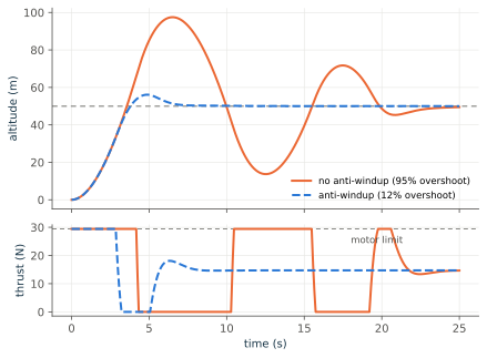
The fix in the lab is conditional integration. Accept the new integral value unless the output is at a limit and the error is pushing further into that limit. It takes three lines of code, and it is the difference between a drone that levels off and one that climbs about 47 m past its target.

G. The car: a bicycle with a steering wheel#

Collapse a car’s four wheels into two, one rear and one front, a wheelbase $L$ apart. Track the rear axle at $(x,y)$ with heading $\psi$, speed $v$, and front-wheel angle $\delta$. The kinematic bicycle model is

The first two equations split velocity into components (the unit-circle $\cos$ and $\sin$ from Module 04). The third says the car turns faster when it drives faster or steers harder.

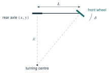
Holding the steering at $\delta$ drives the rear axle around a circle of radius $R=L/\tan\delta$.

Hold $\delta$ constant and the car traces a circle. The right triangle formed by the rear axle, the front wheel, and the turning centre gives $\tan\delta=L/R$, so $R=L/\tan\delta$. For a 2.9 m wheelbase and $\delta=5^\circ$, $R\approx33.1$ m. The lab’s circle test confirms the simulation stays on that radius.

H. Pure pursuit: steer toward a carrot on the path#

Pure pursuit is a classic path-following method in robotics, and a standard baseline for any learned controller. Pick a point on the path a fixed look-ahead distance $\ell$ ahead of the car (the carrot). Then steer along the one circle that passes through the rear axle, is tangent to the current heading, and reaches the carrot.

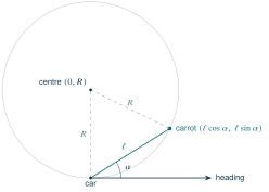
Put the car at the origin facing $+x$. The circle it can drive, tangent to the heading, has its centre at $(0,R)$.

The derivation is a single line of Algebra First. The circle is $x^2+(y-R)^2=R^2$. The carrot sits at $(\ell\cos\alpha,\ \ell\sin\alpha)$. Substitute and expand:

The bicycle model turns curvature into a steering angle, $\tan\delta=L\kappa$, so

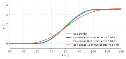
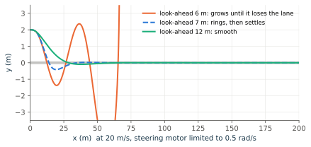
The look-ahead distance is the one tuning knob, and it trades two failures against each other. A short look-ahead reacts fast and hugs corners, but with a steering motor that turns the wheels at only 0.5 rad/s, it overcorrects and rings. At 6 m the ringing grows until the car loses the lane. A long look-ahead is smooth but cuts corners: on a lane change, the worst error grows from 2 cm at 4 m to 34 cm at 16 m. Production systems usually scale look-ahead with speed.

I. A real bug, and why it became a test#

The first version of this lab searched the entire path for the closest point on every tick. It worked on straight roads and lane changes, then failed on a 1.5-lap circle. As the car passed the top of the loop, the closest segment was the one from the second lap, lying exactly on top of the first. The look-ahead search started from the end of the path, the carrot collapsed onto the car, and the car spun in a tight circle.

The fix was a bounded search: look only a short distance ahead of the previous closest segment. A regression test, test_tracks_a_looping_path, now drives the loop so the bug cannot quietly return. This is what debugging looks like on autonomy teams. Find the scenario the method assumed away, prove the failure, fix the smallest thing, and pin it with a test.

J. Where this shows up in real stacks#

• Drones. PX4’s multicopter controller is a cascade of loops: position feeds velocity, velocity feeds attitude, and attitude feeds angular rate. Each loop is a P or PID controller like the one above, running inside the flight stack alongside the EKF2 estimator. ArduPilot follows the same pattern with EKF3.
• Self-driving. Tesla’s FSD now maps camera pixels to driving controls with one end-to-end network rather than hand-written planning code. Engineers still judge any controller, learned or not, with this chapter’s vocabulary: stability, overshoot, saturation, delay, and steady-state error. Pure pursuit and PID remain standard baselines and fallbacks throughout robotics.
• Game engines. A game’s fixed-step simulation, such as a physics loop ticking at 64 Hz, runs the same measure–compare–act loop every tick. Porting this lab into C++ inside a game engine, with live plots, is the portfolio step at the end of this chapter.

K. The lab#

The lab ships with its starters and tests in the companion code’s frontier_code folder (bezhig.com/book). It needs only Python’s standard library. starters/control_lab.py has three blanks: PID.update (F01.L1), bicycle_step (F01.L2), and pure_pursuit_steer (F01.L3). Each docstring gives the recipe. Fill them in, then run the same 20 tests used for the reference solution:

cd frontier_code
$env:MANUAL_IMPL = "starters"          # PowerShell
python -m unittest discover -s tests -p "test_*.py" -v

In bash or zsh, set the variable with export MANUAL_IMPL=starters instead. Three of the tests each pin one idea from this chapter:

• test_no_derivative_kick_on_setpoint_jump (section E),
• test_integral_frozen_while_saturated… (section F),
• test_tracks_a_looping_path (section I).

When one fails, read its name and the section it points to before touching the code.

L. Independent practice#

F foundation C standard course work T transfer S optional stretch L runnable lab or project. Attempt the complete set before opening its solutions.

M. Complete solutions: F01#

Compare the first step where your work differs. A corrected answer is not yet an independent success.

Open every solution

N. Retention and readiness#

Explain aloud, without notes, why P-only control stalls at $mg/K_P$, and derive pure-pursuit curvature from $x^2+(y-R)^2=R^2$. Revisit M12.05 and F01.04 together: both differentiate a geometric relationship before substituting. Log any F01 error under its error family from LM (Part I). Advance to the next Frontier chapter when all 20 lab tests pass on your own starter code.