A04: Statistics, experiments, and uncertainty in measurements

A. Prerequisites and observable goals#

Level: Degree core; introductory inference, not a full statistics specialization.

B. The central question: what does a finite sample justify?#

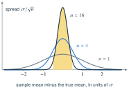
A sample is observed data. A parameter is a property of a specified population or model. An estimator is a rule that computes a proposed parameter value from a sample. For independent identically distributed observations with finite variance $\sigma^2$, the sample mean $\bar X$ has expectation $\mu$ and variance $\sigma^2/n$. Averaging reduces this kind of sampling variability, but it does not remove systematic measurement error, selection bias, or an incorrect model.

Measuring only successful requests estimates latency conditional on success, not latency and reliability for all attempted requests. Measuring only after caches are warm describes a warm-cache workload. Discarding slow observations because they “look like noise” can erase precisely the tail that users experience. Define the population, workload, inclusion policy, and units before collecting results.

C. Confidence intervals quantify a procedure, not certainty about one interval#

When the population variance is known and normality holds, or an appropriate large-sample approximation is justified,

is a familiar approximate 95% confidence interval for a mean. When variance is estimated from an independent normal sample, use a Student $t$ critical value with $n-1$ degrees of freedom and standard error $s/\sqrt n$. The small-sample $t$ result relies on its assumptions; replacing every difficult latency distribution with a normal one is not justified by notation.

The frequentist 95% statement concerns repeated samples and the interval-building procedure: under the assumptions, 95% of such intervals cover the fixed parameter. It does not mean 95% of observations lie inside this interval, and it is not automatically a 95% posterior probability that the parameter lies in this particular realized interval. A prediction interval for a future observation is a different object and usually wider. A Bayesian credible interval answers another question after specifying a prior and likelihood.

The central limit theorem explains why normalized sample means can approach a normal distribution under appropriate independence and moment conditions. It is an asymptotic theorem, not a guarantee that any sample of size 30 is adequate. Heavy tails, strong dependence, or nonstationary workloads require more care. [PROB][NIST]

D. Paired measurements preserve the comparison#

Compare an old and new implementation on the same workload instance, and define $d_i=\text{old}_i-\text{new}_i$ in milliseconds. Positive values favor the new implementation. Workload difficulty affects both measurements, so pairing can remove some shared variation. Randomize or alternate execution order to reduce systematic warmup and drift effects. Pairing does not eliminate thermal, scheduling, or order effects automatically.

For differences $10,8,12,10$ ms, the mean reduction is 10 ms. The sample variance is $(0^2+(-2)^2+2^2+0^2)/3=8/3\ \mathrm{ms}^2$, so the standard error is $\sqrt{8/3}/2\approx0.8165$ ms. Using the supplied two-sided 95% $t$ critical value 3.182 for three degrees of freedom gives approximately $10\pm2.60$ ms. The result is conditional on independent approximately normal pair differences. Four pairs are weak evidence for diagnosing an arbitrary real latency distribution; the example teaches the calculation, not a recommended universal sample size.

A bootstrap resamples observed pairs with replacement, computes the statistic for each resample, and uses the distribution of those statistics to approximate sampling uncertainty. Resampling old and new values independently would destroy pairing. A simple percentile interval can be inaccurate in small samples or biased/skewed settings. Correlated time-series observations may require block-based methods rather than treating each request as an independent draw. The lab explicitly uses the simpler independent-pairs model.

E. Hypothesis tests do not measure the probability that a hypothesis is true#

A null hypothesis might specify zero mean paired difference. A test statistic measures how incompatible the observation is with the null model. A $p$-value is the probability, under that null model and its assumptions, of obtaining a result at least as extreme according to the test’s rule. It is not $P(\text{null is true}\mid\text{data})$ and not the probability that the result was “caused by chance.” Failing to reject does not prove equality or practical equivalence. Equivalence requires a specified tolerance and an appropriate analysis.

Effect size asks how much changed: milliseconds saved, error rate reduced, or a standardized difference. A huge sample can make a tiny, unimportant difference statistically detectable. A small sample can leave a practically important difference uncertain. Report an effect estimate with uncertainty and the engineering requirement it is meant to satisfy. “Statistically significant” and “fast enough” answer different questions.

Multiple attempts change the evidence. If 20 independent null tests each use a 5% false-positive rate, the probability of at least one false rejection is $1-0.95^{20}\approx0.642$. Repeatedly tuning on the test set and reporting only the best outcome is another form of selection. Predeclare the main comparison, retain failed trials, and use separate validation and final evaluation data when developing models or choosing configurations.

F. Regression and causal claims#

Linear regression models a response as $y=\beta_0+\beta_1x+\varepsilon$. Least squares estimates coefficients by minimizing a specified loss. Its geometric solution does not itself establish that increasing $x$ causes $y$ to change. A confounder may influence both. For example, more powerful devices might both select higher graphics settings and achieve higher frame rates; an observational positive association does not prove that raising graphics quality improves speed.

A randomized controlled comparison assigns conditions independently of potential outcomes, subject to practical design constraints. Blocking by device or workload and pairing repeated runs can improve precision. Blind evaluation, fixed metrics, and a documented exclusion policy reduce opportunities for accidental bias. Privacy and consent remain relevant when measurements come from people rather than synthetic fixtures. In this book, all fixtures are synthetic and no real customer data is used.

G. Independent practice#

F foundation C standard course work T transfer S optional stretch L runnable lab or project. Attempt the complete set before opening its solutions.

H. Complete solutions: A04#

Compare the first step where your work differs. A corrected answer is not yet an independent success.

Open every solution

"""A04.05: paired bootstrap of mean change. An approximation, not a guarantee."""
import math
import random
import statistics

def paired_bootstrap(before: list[float], after: list[float],
                     repetitions: int = 2000, seed: int = 42) -> dict:
    if len(before) != len(after) or len(before) < 2:
        raise ValueError("at least two matched pairs required")
    if any(not math.isfinite(x) for x in before + after):
        raise ValueError("finite observations required")
    if type(repetitions) is not int or repetitions < 100:
        raise ValueError("at least 100 resamples required")
    differences = [b - a for b, a in zip(before, after)]
    rng = random.Random(seed)
    n = len(differences)
    means = sorted(statistics.mean(rng.choices(differences, k=n))
                   for _ in range(repetitions))
    lo = means[math.ceil(0.025 * repetitions) - 1]
    hi = means[math.ceil(0.975 * repetitions) - 1]
    return {"mean_reduction": statistics.mean(differences),
            "percentile_95_interval": [lo, hi],
            "pairs": n, "resamples": repetitions, "seed": seed}

if __name__ == "__main__":
    print(paired_bootstrap([10, 13, 12, 15, 11], [8, 10, 10, 11, 10]))

I. Retention and readiness#

Retrieve the distinction between expectation and an observed value, and between covariance and independence. Advance when you can explain a confidence interval without turning it into an observation range or posterior probability, and can defend an experiment’s sampling and exclusion policy.