A06: Differential equations, stability, and optimization

A. Prerequisites and observable goals#

Level: Degree core with advanced continuation boundaries.

B. The central question: how does a local rule determine an evolving system?#

An initial-value problem specifies a derivative rule $y'(t)=f(t,y(t))$ and an initial state $y(t_0)=y_0$. The solution is a function of time satisfying both. It is not obtained by treating the derivative as an ordinary variable and guessing arbitrary constants. Existence and uniqueness require conditions; continuity of $f$ and a suitable local Lipschitz condition in the state give a standard local result. A numerical trajectory is an approximation to that model, not proof that the model describes the real world.

A second-order equation becomes a first-order vector system. For the dimensionless oscillator $x''=-x$, define $v=x'$. Then

The exact solution is $(\cos t,-\sin t)$. Verify it by differentiating and checking the initial state. Its energy $E=(x^2+v^2)/2$ is constant because $E'=xx'+vv'=xv+v(-x)=0$. These analytical facts provide independent validation targets for a numerical solver.

C. Euler’s method is a tangent approximation in time#

For step $h>0$, explicit Euler uses

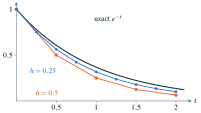
The increment has the state’s units because derivative units multiplied by time give state units. For $y'=-y$, $y(0)=1$, and $h=0.1$, the first values are $1,0.9,0.81$. The exact value at $t=0.2$ is $e^{-0.2}\approx0.818731$. Euler is close over this short interval but not exact. Under appropriate smoothness and stability conditions, the local truncation error is $O(h^2)$ and the accumulated global error over a fixed interval is $O(h)$. Local and global orders are not interchangeable.

D. RK4 samples several slopes, but does not eliminate all error#

Classical fourth-order Runge–Kutta computes

Here each $k_i$ is a derivative, not an already multiplied step increment. Some textbooks define $k_i$ with $h$ included; either convention can work, but mixing them multiplies by $h$ twice. For sufficiently smooth problems over a fixed interval and appropriate step sizes, global error is $O(h^4)$. Halving $h$ should then reduce the dominant error by approximately $2^4=16$, until rounding or another error source dominates. This is an asymptotic diagnostic, not an exact ratio for every step size.

E. Stability asks whether numerical error is amplified#

For $y'=-\lambda y$ with $\lambda>0$, Euler gives $y_{n+1}=(1-\lambda h)y_n$. The exact solution decays, so a basic numerical stability requirement is $|1-\lambda h|<1$, or $0<h<2/\lambda$. With $\lambda=1000$ and $h=0.003$, the multiplier is $-2$, so the numerical values alternate and grow even though the exact solution decays. This is not a sign that the physical model suddenly became unstable.

For the undamped oscillator, Euler gives $(x_{n+1},v_{n+1})=(x_n+hv_n,v_n-hx_n)$. Its energy satisfies

Therefore it adds energy at every positive step. A smaller step reduces finite-time error but does not make explicit Euler a long-term energy-preserving oscillator integrator. Symplectic methods, implicit methods, adaptive error control, and stiffness are important continuation topics. T05 introduces velocity Verlet for a bounded conservative model rather than pretending that one solver is best for all equations.

F. Optimization is an iterative computation with its own conditions#

To minimize a differentiable objective $F(x)$, gradient descent uses $x_{k+1}=x_k-\alpha\nabla F(x_k)$. The negative gradient is a local steepest-descent direction in the Euclidean norm, but a step that is too large can increase the objective. For $F(x)=\frac12\lambda x^2$, the update is $x_{k+1}=(1-\alpha\lambda)x_k$, so convergence to zero requires $0<\alpha<2/\lambda$. The resemblance to the Euler stability calculation is meaningful: both are iterative amplification analyses.

For a positive-definite quadratic $F(x)=\frac12x^TAx-b^Tx$, the gradient is $Ax-b$. A constant step less than $2/\lambda_{\max}(A)$ gives convergence in exact arithmetic, while a wide eigenvalue spread can make it slow. Feature scaling and preconditioning can change the geometry. For nonconvex objectives, a zero gradient need not indicate a global minimum.

Newton optimization solves $H(x_k)p_k=-\nabla F(x_k)$ for a step and then updates $x_{k+1}=x_k+p_k$, possibly with a line search or damping. This is not the same notation as scalar root finding, though it applies root finding to the gradient. An indefinite Hessian can yield a non-descent direction. Do not explicitly invert a large Hessian just because the mathematical formula can be written with $H^{-1}$.

For a box constraint, projected gradient descent replaces the unconstrained trial point by its Euclidean projection onto the box, componentwise clipping. General constraints need more analysis. Lagrange multipliers give necessary conditions under suitable regularity, not automatic global optimality. Module 38 supplies the geometric constrained-optimization foundation. The lab in this module focuses on ODE integration; optimization is exercised analytically here and computationally in T03.

G. Independent practice#

F foundation C standard course work T transfer S optional stretch L runnable lab or project. Attempt the complete set before opening its solutions.

H. Complete solutions: A06#

Compare the first step where your work differs. A corrected answer is not yet an independent success.

Open every solution

"""A06.05: fixed-step Euler and RK4 for finite-dimensional ODE systems."""
import math
from collections.abc import Callable

def integrate(f: Callable, y0: tuple[float, ...], t0: float, t1: float,
              steps: int, method: str = "rk4") -> list[tuple[float, tuple]]:
    if type(steps) is not int or steps < 1 or not y0:
        raise ValueError("positive integer steps and nonempty state required")
    if not all(math.isfinite(x) for x in (t0, t1, *y0)) or t1 <= t0:
        raise ValueError("finite data and increasing time required")
    if method not in {"euler", "rk4"}:
        raise ValueError("unknown integration method")
    h = (t1 - t0) / steps
    y = tuple(float(x) for x in y0)
    out = [(t0, y)]
    def derivative(t, state):
        d = tuple(f(t, state))
        if len(d) != len(y0) or any(not math.isfinite(x) for x in d):
            raise ValueError("invalid derivative shape or value")
        return d
    def add(state, d, factor):
        return tuple(a + factor * b for a, b in zip(state, d))
    for i in range(steps):
        t = t0 + i * h
        k1 = derivative(t, y)
        if method == "euler":
            y = add(y, k1, h)
        else:
            k2 = derivative(t + h / 2, add(y, k1, h / 2))
            k3 = derivative(t + h / 2, add(y, k2, h / 2))
            k4 = derivative(t + h, add(y, k3, h))
            y = tuple(v + h * (a + 2*b + 2*c + d) / 6
                      for v, a, b, c, d in zip(y, k1, k2, k3, k4))
        if any(not math.isfinite(x) for x in y):
            raise ArithmeticError("nonfinite integration state")
        out.append((t0 + (i + 1) * h, y))
    return out

if __name__ == "__main__":
    path = integrate(lambda t, y: (-y[0],), (1.,), 0., 1., 10)
    print(path[-1], "exact:", math.exp(-1))

I. Retention and readiness#

Retrieve the tangent-line approximation, the chain rule, and eigenvalue growth. Advance when you can distinguish local error, global error, stability, and modeling error, and when a solver’s output comes with an analytical or conservation-based check rather than a claim that the plot looks right.