G12: Machine learning objectives, generalization, and decisions

Prerequisites and observable goals#

The central question: what is learned, from which evidence?#

A learning algorithm maps a training dataset to model parameters. A fitted model maps an input to a prediction. A decision policy maps that prediction to an action. These are three different functions with different failure modes. A low training loss says the first function found parameters that fit observed examples; it does not prove the prediction will transfer or that the action is justified.

Write a dataset $\{(x_i,y_i)\}_{i=1}^n$, where $x_i\in\R^d$ and $y_i\in\{0,1\}$. The index $i$ identifies an example; the feature coordinate $j$ identifies a component. In the lab, rows are examples and weights are a length-$d$ vector. The empirical objective is an average of losses, possibly plus a regularizer:

The bias $b$ is deliberately not penalized. A different convention is possible but changes the derivatives and the fit. The target quantity for generalization is an expectation over the intended future population, not merely this finite average. Describe that population and the available evidence for sampling it. Stanford’s CS229 notes provide a primary course treatment of supervised objectives and classification. The numerical examples here are original. [G-ML]

Derive a stable binary objective#

Let the logit be $z=w^Tx+b$ and probability $p=\sigma(z)=1/(1+e^{-z})$. The logit ranges over real numbers; the probability is in $(0,1)$ in exact arithmetic. These objects are not interchangeable. A Bernoulli likelihood for target $y$ is $p^y(1-p)^{1-y}$. Taking its negative logarithm gives

The last expression avoids calculating two logs of probabilities but can still overflow when $z$ is large. Use the algebraically equivalent form

Implement the last logarithm with log1p. For $z=-1000,y=1$, the loss is approximately 1000, not NaN. A numerically saturated sigmoid of zero does not mean the mathematical likelihood model assigned an exact impossible event.

For $z\ge0$, compute the sigmoid directly using $e^{-z}$; for $z<0$, use $e^z/(1+e^z)$. Each branch avoids exponentiating a large positive value. This is a numerical implementation choice, not a new statistical model.

The derivative is a sensitivity, not a probability#

Differentiate the logit form:

By the chain rule, $\partial z/\partial w_j=x_j$ and $\partial z/\partial b=1$. Therefore

The gradient has one component per parameter. It is not the vector of predictions and not an instruction to change the inputs. A gradient-descent update subtracts a learning-rate multiple of that gradient from the parameters, holding the training examples fixed.

Worked one-example step: $x=2,y=1,w=0,b=0,\lambda=0$. Then $z=0$, $p=1/2$, loss $\log2$, weight gradient $(-1/2)(2)=-1$, and bias gradient $-1/2$. With learning rate $.1$, the simultaneous new parameters are $w=.1,b=.05$. The new logit is $.25$, probability about $.56218$, and loss about $.57594$, smaller than $.69315$. Compute both updates from the old state; updating one parameter before calculating the other can implement a different algorithm.

Curvature explains part of the optimization behavior#

With an augmented input $\widetilde x=(x,1)$ and parameter vector $\theta=(w,b)$, the data Hessian is

For any direction $v$, its quadratic form is $n^{-1}\sum_i p_i(1-p_i)(\widetilde x_i^Tv)^2\ge0$. Thus the data objective is convex in these linear-model parameters. Adding nonnegative L2 regularization preserves convexity. Positive definiteness and uniqueness require more conditions, especially because the bias is unpenalized.

On linearly separable observations, unregularized logistic loss can decrease as the weight norm grows without attaining a finite minimizer. A decreasing training curve is not evidence that parameters will converge to a bounded value. Regularization changes the objective and may control this growth; its strength must be selected without inspecting the final test outcomes.

Newton-type methods use curvature to choose a step by solving a linear system rather than literally forming an inverse. Damping or a line search can help control unsuitable steps. G05 explains conditioning; nearly dependent features can make curvature calculations difficult. The reference deliberately uses simple gradient descent so the state changes and derivatives remain inspectable, not because it is universally optimal.

Fitting, selection, and evaluation are separate stages#

Training data fits weights and preprocessing. Validation data chooses features, hyperparameters, thresholds, or stopping rules. Test data estimates the behavior of the frozen choice on the declared evaluation unit. If one user’s sessions appear in both training and test, the measurement may describe memorization of known users rather than performance on new users. Split by group when new groups are the intended target; split by time when forecasting the future. Neither split universally replaces the other.

Fit a scaler only on training rows; retain its parameters and apply them unchanged. Repeatedly comparing dozens of configurations on a validation set can overfit that set too. A final held-out set is not a renewable source of independent evidence after every design change. GP2 records a deliberately small predeclared candidate set and evaluates the test only after selection. Rerunning the same deterministic experiment reproduces the computation; it does not create another independent dataset.

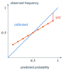
Accuracy can obscure rare-class failures. Log loss measures probability assignments; Brier score measures squared probability error; precision and recall describe threshold decisions. Report counts and class balance. Calibration asks whether outcomes occur at frequencies consistent with predicted probabilities in a specified population and grouping procedure. Good discrimination does not automatically imply good calibration.

From probabilities to actions#

Suppose correct actions have cost zero, a false positive costs $C_{FP}>0$, and a false negative costs $C_{FN}>0$. If $p$ is the relevant posterior probability, the expected cost of a positive decision is $C_{FP}(1-p)$; the negative decision costs $C_{FN}p$. Choose positive when

This derivation explains why $.5$ is not a universal threshold. It depends on calibrated probabilities for the use population, suitable cost assumptions, and a legitimate decision policy. Review capacity, abstention, uncertainty, and stakeholder concerns can require a different design. Cost arithmetic does not settle the ethics in G11.

Machine learning is also not all of AI. Search uses explicit states and transitions, planning uses action consequences, and reinforcement learning uses rewards and state distributions affected by a policy. For a discounted finite Markov decision process, the Bellman optimality expression is $V(s)=\max_a[r(s,a)+\gamma\sum_{s'}P(s'\mid s,a)V(s')]$ with $0\le\gamma<1$. For a self-looping state receiving reward 1 every step and $\gamma=1/2$, the fixed point is $V=1+V/2=2$. This is a controlled model calculation, not permission to deploy a learned controller. Further reinforcement-learning study requires the modeling and evaluation assumptions that this supervised lab does not cover.

Independent practice#

F foundation C standard course work T transfer S optional stretch L runnable lab or project. Attempt the complete set before opening its solutions.

Smallest useful hints#

For .02, differentiate $\lambda(w_1^2+w_2^2)/2$. For .04, compare two expected costs before inserting the numbers. For .05, first ask what happens if every prediction is negative.

Complete solutions: G12#

Compare the first step where your work differs. A corrected answer is not yet an independent success.

Open every solution

"""G12: from-scratch binary logistic regression; no external dependencies."""
import math


def validate_xy(X, y):
    n, d = len(X), len(X[0]) if X else 0
    if not 1 <= n <= 10000 or not 1 <= d <= 64 or len(y) != n:
        raise ValueError("bounded nonempty samples/features and matching labels required")
    if any(len(row) != d for row in X):
        raise ValueError("ragged feature matrix")
    if any(type(v) is not int or v not in (0,1) for v in y):
        raise ValueError("strict 0/1 labels required")
    if any(not math.isfinite(v) for row in X for v in row):
        raise ValueError("finite features required")
    return n, d


def sigmoid(z):
    if not math.isfinite(z):
        raise ValueError("finite logit required")
    if z >= 0:
        return 1/(1+math.exp(-z))
    e = math.exp(z)
    return e/(1+e)


def logit_loss(z, y):
    if not math.isfinite(z) or type(y) is not int or y not in (0,1):
        raise ValueError("finite logit and strict binary target required")
    return max(z, 0.) - y*z + math.log1p(math.exp(-abs(z)))


def loss_gradient(w, b, X, y, lam=0.):
    n, d = validate_xy(X, y)
    if len(w) != d or not all(math.isfinite(v) for v in [*w,b,lam]) or lam < 0:
        raise ValueError("valid parameters and nonnegative regularization required")
    loss, grad, db = 0., [0.]*d, 0.
    for row, target in zip(X,y):
        z = math.fsum(a*v for a,v in zip(w,row)) + b
        loss += logit_loss(z,target)/n
        error = (sigmoid(z)-target)/n
        db += error
        for j in range(d):
            grad[j] += error*row[j]
    loss += .5*lam*math.fsum(v*v for v in w)
    grad = [g+lam*v for g,v in zip(grad,w)]
    if not all(math.isfinite(v) for v in [loss,*grad,db]):
        raise ValueError("nonfinite loss/gradient: check scale")
    return loss, grad, db


def fit(X, y, lam=.01, rate=.1, steps=400):
    _, d = validate_xy(X,y)
    if type(steps) is not int or not 1 <= steps <= 10000 or not math.isfinite(rate) or rate <= 0:
        raise ValueError("bounded positive step count and rate required")
    w,b = [0.]*d,0.
    for _ in range(steps):
        _,gw,gb = loss_gradient(w,b,X,y,lam)
        w = [a-rate*g for a,g in zip(w,gw)]
        b -= rate*gb
    final,_,_ = loss_gradient(w,b,X,y,lam)
    return {"weights":w, "bias":b, "objective":final}


def predict(model, X):
    w,b = model["weights"],model["bias"]
    if not w or not all(math.isfinite(v) for v in [*w,b]):
        raise ValueError("invalid model")
    if any(len(row) != len(w) or any(not math.isfinite(x) for x in row) for row in X):
        raise ValueError("invalid feature shape or value")
    return [sigmoid(math.fsum(a*x for a,x in zip(w,row))+b) for row in X]


if __name__ == "__main__":
    X,y = [[-2.],[-1.],[1.],[2.]],[0,0,1,1]
    model = fit(X,y)
    print(model)
    print(predict(model,X))

Readiness and continuation#

Explain every dimension in the gradient and why a test sample must not fit the scaler. Then implement the same objective with a framework and compare outputs, gradients, and reduction conventions before trusting convenience APIs. Further study includes kernels, statistical learning theory, probabilistic modeling, calibrated uncertainty, and reinforcement learning. These require additional problem solving, not just a larger model.