Module 23: Numerical integration and honest error bounds

8 exercises, each with a complete solution. 1 figure. 1 note from the engine.

On this page

A. Prerequisites and observable goals
B. The central idea: finite data can approximate accumulation
C. Composite rules and sufficient error assumptions
D. Why the weights and rates differ
E. A computation procedure
F. Worked examples
Computing bridge: An error budget is part of the specification
G. Independent practice
H. Complete solutions: Module 23
I. Retention and readiness

A. Prerequisites and observable goals#

Before

Definite integrals, finite sums, higher derivatives, and inequalities.

After

Compute composite midpoint, trapezoidal, and Simpson approximations; distinguish actual error from a bound; and select a mesh meeting a stated guarantee.

B. The central idea: finite data can approximate accumulation#

A definite integral is a limiting object, but a computer or table supplies finitely many values. Numerical quadrature replaces the curve by simple pieces: rectangles, line segments, or parabolas. Increasing the sample count often improves accuracy, but a reliable error claim needs hypotheses about the function between the samples. Values at a few nodes alone cannot rule out a narrow spike that every sample missed.

Two ways to replace the curve. Left: chords between the samples give two trapezoids with total area

3.4564

. Right: one parabola through the same three samples (Simpson’s rule) gives

3.2104

. The exact area under

y=\tfrac12e^x

[0,2]

3.1945

, so from the same three samples Simpson’s error is about one sixteenth of the trapezoids’.

C. Composite rules and sufficient error assumptions#

For equal spacing $h=(b-a)/n$ , $x_i=a+ih$ , define

M_n=h\sum_{i=1}^n f\bigl(a+(i-\tfrac12)h\bigr),

T_n=\frac h2\left[f(x_0)+2\sum_{i=1}^{n-1}f(x_i)+f(x_n)\right].

For even $n$ , the composite Simpson rule is

S_n=\frac h3\left[f(x_0)+4\!\sum_{\substack{1\le i<n\\i\text{ odd}}}f(x_i) +2\!\sum_{\substack{2\le i<n\\i\text{ even}}}f(x_i)+f(x_n)\right].

If $f\in C^2[a,b]$ and $|f''|\le K_2$ , sufficient absolute error bounds are

|I-M_n|\le\frac{K_2(b-a)^3}{24n^2},\qquad |I-T_n|\le\frac{K_2(b-a)^3}{12n^2}.

If $f\in C^4[a,b]$ and $|f^{(4)}|\le K_4$ , then for even $n$ ,

|I-S_n|\le\frac{K_4(b-a)^5}{180n^4}.

These are upper bounds, not predictions of the exact error, and $K_2,K_4$ must bound derivatives on the entire interval. Standard rules and error estimates: [O2Num].

D. Why the weights and rates differ#

A trapezoid of width $h$ and endpoint heights $f(x_i),f(x_{i+1})$ has area $h[f(x_i)+f(x_{i+1})]/2$ . Adding adjacent trapezoids counts interior heights twice, giving the weights $1,2,\ldots,2,1$ .

Simpson’s rule integrates the quadratic interpolating each pair of subintervals, producing weights $1,4,1$ across three nodes. Joining pairs makes shared interior even nodes carry weight $2$ . This explains both the even- $n$ requirement and why the rule is exact for quadratic polynomials; symmetry also makes it exact for cubics. The error powers arise because the local interpolation errors accumulate over the mesh. The displayed bounds include the constants; a vague statement “fourth-order accuracy” does not itself give a numerical guarantee.

E. A computation procedure#

Record $a,b,n,h$ and confirm equal spacing. Write a node-and-value table. Apply the correct weights, sum before rounding aggressively, and multiply by the width factor last. To meet a tolerance, solve the appropriate error inequality for $n$ and round upward; for Simpson, round upward to an even integer. Check that the function is smooth enough and that its derivative bound is valid. A singular endpoint requires a different analysis or a change of variable, not blind use of these bounds.

F. Worked examples#

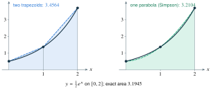
A trapezoidal approximation. For $\int_0^1e^x\dd x$ with $n=2$ , $h=1/2$ and

T_2=\frac14(1+2\sqrt e+e)\approx1.75393.

The exact value is $e-1\approx1.71828$ , so the error is about $0.03565$ . Since $f''=e^x\le e$ on $[0,1]$ , the bound is $e/48\approx0.05663$ , larger than the actual error, as a valid upper bound should be.

A guaranteed mesh. For the same integral, a trapezoidal error at most $10^{-4}$ is guaranteed by $e/(12n^2)\le10^{-4}$ , giving $n\ge\sqrt{e/(0.0012)}\approx47.60$ . Thus $n=48$ suffices. It is not necessarily the smallest mesh that happens to meet the tolerance; it is the smallest integer certified by this particular bound.

Implementation connection. A game simulation’s accumulated movement from sampled velocities resembles quadrature. A trapezoidal update averages endpoint velocities; it is not identical to knowing the exact continuous trajectory. Time-step error, model error, and floating-point error are separate sources of discrepancy.

Computing bridge: An error budget is part of the specification#

A numerical result without a workload and an error condition is incomplete. Simpson’s rule has a theorem-based bound only when the fourth derivative is bounded on the integration interval and the panel count is valid. A05 implements that composite formula and compares it with an analytically known answer. A test using a cubic should be exact up to floating-point effects; that success alone does not establish accuracy for an oscillatory or nonsmooth integrand. Match the regularity assumptions before reusing the bound.

From the engine: NightjarAn integral that reports its own error

Nightjar integrates a probability density to find the chance that two satellites collide, and there an answer without an error estimate would be useless. Its integrator evaluates the function at 15 points. All 15, weighted one way, give a Kronrod estimate; seven of the same points, weighted another way, give a 7-point Gauss estimate at no extra cost.

Nightjar: a Gauss--Kronrod panelC++

QuadratureEstimate gk15(F&& f, double lo, double hi) {
    const double centre = 0.5 * (lo + hi);
    const double half = 0.5 * (hi - lo);
    const double fc = f(centre);
    double kronrod = fc * kWgk[7];
    double gauss = fc * kWg[3];
    for (int j = 0; j < 7; ++j) {
        const double dx = half * kXgk[static_cast<std::size_t>(j)];
        const double pair = f(centre - dx) + f(centre + dx);
        kronrod += kWgk[static_cast<std::size_t>(j)] * pair;
        if (j % 2 == 1) gauss += kWg[static_cast<std::size_t>(j / 2)] * pair;
    }
    return {kronrod * half, std::fabs((kronrod - gauss) * half)};
}

The Gauss rule is exact for polynomials through degree 13 and the Kronrod rule through degree 23, so where the function is smooth the two agree closely. Their difference, the second value returned, is an estimate of the error, and usually a pessimistic one. Try one panel on $1/(1 + x^2)$ from 0 to 4, whose integral is $\arctan 4 \approx 1.3258177$ . The Kronrod value is off by $2.3\times 10^{-9}$ , and the estimate returned is $6.5\times 10^{-5}$ : it is really the error of the 7-point rule, so it overstates the error of the value it travels with by four orders of magnitude. An estimate is still not a guarantee, as this module’s error bounds are: a function that happened to vanish at all fifteen points would return zero for both. The module’s theme is the same either way: report the number together with a statement of how far to trust it. The routine that calls this one, not shown, is adaptive: it splits the panel with the largest estimate at its midpoint and repeats until the total meets the tolerance.

G. Independent practice#

F foundation C standard course work T transfer S optional stretch L runnable lab or project. Attempt the complete set before opening its solutions.

M23.01FSolution

Compute $M_2$ and $T_2$ for $\int_0^2x^2\dd x$ , and compare their errors with the exact integral.

M23.02CSolution

Compute $S_4$ for $\int_0^2x^3\dd x$ . Explain the exact agreement.

M23.03CSolution

For $\int_0^1e^x\dd x$ , choose the smallest even $n$ guaranteed by the Simpson bound to give error at most $10^{-6}$ .

M23.04TSolution

A rate table at times $0,1,2,3,4$ seconds gives $v=0,2,3,2,0$ m/s. Find $T_4$ and $S_4$ . Do the data prove either answer exact?

M23.05CSolution

Find a sufficient trapezoidal subinterval count for error at most $0.001$ in $\int_0^\pi\sin x\dd x$ .

M23.06TSolution

Why is the displayed Simpson error bound not automatically applicable to $\int_0^1\sqrt x\dd x$ , even though the integral is finite?

M23.07TSolution

A nonconstant twice differentiable function has $f''>0$ on $[a,b]$ . Explain geometrically the error signs for midpoint and trapezoidal approximations.

M23.08SSolution

Show that five values at the nodes $0,1/4,1/2,3/4,1$ cannot by themselves bound the integral error. Construct nonnegative smooth functions zero at all five nodes with arbitrarily large integrals.

Optional small hints

For M23.03, take a fourth root, then enforce parity. For M23.08, square a polynomial with those five roots and multiply by a positive scale.

H. Complete solutions: Module 23#

Compare the first step where your work differs. A corrected answer is not yet an independent success.

M23.01Show solution

Two rectangle heights versus three endpoint heights

With $h=1$ , midpoint inputs are $1/2,3/2$ , so $M_2=1/4+9/4=\boxed{5/2}$ . Trapezoidal weights give $T_2=(1/2)[0+2(1)+4]=\boxed3$ . The exact integral is $8/3$ . Thus midpoint error magnitude is $1/6$ (underestimate), and trapezoidal error is $1/3$ (overestimate). Here $K_2=2$ makes the corresponding theoretical bounds exactly $1/6$ and $1/3$ .

Back to M23.01

M23.02Show solution

Apply the alternating weights correctly

With $h=1/2$ , the values are $0,1/8,1,27/8,8$ . Therefore

S_4=\frac16\left[0+4(1/8)+2(1)+4(27/8)+8\right]=\frac{24}{6}=\boxed4.

The exact integral is $[x^4/4]_0^2=4$ . Since the fourth derivative of this cubic is zero, the Simpson error bound is zero; this explains exactness beyond a numerical coincidence.

Back to M23.02

M23.03Show solution

A tolerance requirement with an even mesh

Here $K_4=e$ and interval length is $1$ . Require $e/(180n^4)\le10^{-6}$ , or $n\ge(e/0.00018)^{1/4}\approx11.09$ . The smallest permissible even integer is $\boxed{12}$ . The bound is then $e/(180\cdot12^4)\approx7.28\times10^{-7}$ , below the target.

Back to M23.03

M23.04Show solution

The table determines approximations, not the missing curve

The width is $1$ . Trapezoidal integration gives $T_4=\tfrac12[0+2(2+3+2)+0]=\boxed7$ m. Simpson gives $S_4=\tfrac13[0+4(2)+2(3)+4(2)+0]=\boxed{22/3}$ m. Neither is proven exact from the table alone; curves between the samples can differ. There is also no derivative bound supplied to certify either error.

Back to M23.04

M23.05Show solution

Round a sufficient count upward

Since $f''=-\sin x$ , $|f''|\le1$ . The bound is $\pi^3/(12n^2)$ . Requiring this at most $0.001$ gives $n\ge\sqrt{\pi^3/0.012}\approx50.83$ , so $\boxed{51}$ subintervals suffice. Trapezoidal rules have no even- $n$ restriction.

Back to M23.05

M23.06Show solution

Integrability is weaker than the error theorem’s hypotheses

The square root is continuous on $[0,1]$ , hence integrable, but its derivatives become unbounded near zero; in particular its fourth derivative has no finite bound on the entire interval. The stated $C^4$ and finite- $K_4$ assumptions fail. This does not say Simpson approximations are meaningless, only that this specific guarantee cannot be invoked without additional analysis.

Back to M23.06

M23.07Show solution

Curvature predicts opposite biases

For a strictly convex graph, each secant chord lies above the curve, so each trapezoid overestimates area. For midpoint rectangles, pair points equally spaced around the midpoint; convexity makes the average of their heights exceed the midpoint height. Integrating those paired comparisons shows the midpoint underestimate. Thus $M_n<I<T_n$ under strict convexity on a nonzero interval. This is an exact sign conclusion, not just a tendency seen in a picture.

Back to M23.07

M23.08Show solution

Unseen behavior can defeat a data-only guarantee

Let $p(x)=x(x-1/4)(x-1/2)(x-3/4)(x-1)$ and $f_K(x)=Kp(x)^2$ with $K>0$ . Every sampled value is zero, so the trapezoidal and Simpson rules on these nodes give zero. But $p^2$ is continuous, nonnegative, and positive except at finitely many roots, so $c=\int_0^1p^2\dd x>0$ . The true integral is $Kc$ , which becomes arbitrarily large. Smoothness alone without a quantitative derivative bound does not prevent the example; all these functions are polynomials.

Back to M23.08

I. Retention and readiness#

Retrieve M16.03 and M15.08. Explain the difference between an observed error, an estimated error, and a proven upper bound. Advance when you can audit someone else’s node spacing, weights, parity, and derivative assumptions.