Module 31: Parametric curves and Cartesian conics

8 exercises, each with a complete solution. 1 figure.

On this page

A. Prerequisites and observable goals
B. The central idea: one input can control two coordinates
C. Calculus with a parameter
D. Why the slope formula is a ratio
E. A geometry-first workflow
F. Worked examples
G. Independent practice
H. Complete solutions: Module 31
I. Retention and readiness

A. Prerequisites and observable goals#

Before

Derivatives, integrals, coordinate geometry, and completing the square.

After

Read a curve’s geometry and orientation from a parameter, compute slopes and lengths, and identify basic conics without losing parameter restrictions.

B. The central idea: one input can control two coordinates#

A parametric curve specifies $x=x(t)$ and $y=y(t)$ on a stated parameter interval. Its output is a point, not just a height. Eliminating $t$ can reveal the underlying geometric curve, but it may lose direction, speed, endpoint restrictions, or repeated tracing. Those features matter in calculus even when two parameterizations draw the same shape.

A parameter adds direction and timing. The path

x=3\cos t

y=2\sin t

for

0\le t\le\tfrac{3\pi}2

traces three quarters of the ellipse

x^2/9+y^2/4=1

, counterclockwise from the green point

(3,0)

to the red point

(0,-2)

. Eliminating

t

gives the whole ellipse and loses where the motion starts, which way it goes, and where it stops.

C. Calculus with a parameter#

For differentiable coordinates, where $x'(t)\ne0$ ,

\frac{\dd y}{\dd x}=\frac{y'(t)}{x'(t)},\qquad \frac{\dd^2y}{\dd x^2}=\frac{\frac{\dd}{\dd t}(y'/x')}{x'(t)}.

The second derivative is not generally $y''(t)/x''(t)$ . A horizontal tangent can occur when $y'=0,x'\ne0$ ; a vertical tangent when $x'=0,y'\ne0$ . If both vanish, examine the limiting geometry instead of dividing zero by zero.

For a smooth curve traced once,

L=\int_\alpha^\beta\sqrt{x'(t)^2+y'(t)^2}\dd t.

The signed integral $\int y\dd x$ becomes $\int_\alpha^\beta y(t)x'(t)\dd t$ . If a parameter reverses direction, signed contributions and arc length behave differently: arc length remains nonnegative and counts all tracing. Parametric calculus: [O2Param].

Standard conics include an ellipse $(x-h)^2/a^2+(y-k)^2/b^2=1$ , a hyperbola with a difference of two positive squared terms, and a parabola such as $(y-k)^2=4p(x-h)$ . For a horizontal ellipse with $a\ge b>0$ , focal distance is $c=\sqrt{a^2-b^2}$ . For a horizontal hyperbola, $c=\sqrt{a^2+b^2}$ and asymptotes are $y-k=\pm(b/a)(x-h)$ . Complete squares and normalize before assigning these parameters.

D. Why the slope formula is a ratio#

Over a small parameter change, coordinate increments are approximately $x'\Delta t$ and $y'\Delta t$ . Their ratio approaches $y'/x'$ when the denominator derivative is nonzero. Differentiating that slope with respect to $x$ requires dividing its $t$ derivative by $x'$ again. Arc length instead measures the magnitude of the displacement vector, giving a square root of the sum of squared coordinate rates.

For a conic, the sign pattern after completing squares determines whether two directions are bounded (ellipse), branches open apart (hyperbola), or one coordinate is quadratic in the other (parabola). A degenerate or empty real locus is possible; a quadratic equation is not automatically a nondegenerate conic.

E. A geometry-first workflow#

Record the parameter interval, find a few ordered points, and mark the direction of increasing $t$ . Eliminate the parameter only when useful, and retain any restrictions. For tangents, evaluate the point and both coordinate derivatives. For arc length, integrate speed and check whether the curve retraces. For a conic equation, group coordinates, complete squares, move constants, and divide into standard form before interpreting axes, foci, or asymptotes.

F. Worked examples#

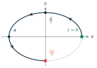
A circle with direction. The parameterization $x=2\cos t,y=2\sin t$ , $0\le t\le2\pi$ , traces the radius-two circle once counterclockwise. Replacing $t$ by $-t$ reverses direction; using $0\le t\le4\pi$ traces twice. Elimination yields $x^2+y^2=4$ in all three cases, but length counted by the parameter and signed integrals differ.

A second derivative. With $x=t^2+1,y=t^3$ and $t>0$ , $\dd y/\dd x=3t/2$ . Its $t$ derivative is $3/2$ , so $\dd^2y/\dd x^2=(3/2)/(2t)=3/(4t)$ . The positivity indicates concavity up on this branch.

Completing squares. For $4x^2+y^2-8x+6y=3$ , rearrange to $4(x-1)^2+(y+3)^2=16$ . Thus $(x-1)^2/4+(y+3)^2/16=1$ : an ellipse centered at $(1,-3)$ with vertical semimajor axis $4$ and horizontal semiminor axis $2$ . The larger denominator identifies the major axis, not the larger coefficient in the original equation.

G. Independent practice#

F foundation C standard course work T transfer S optional stretch L runnable lab or project. Attempt the complete set before opening its solutions.

M31.01FSolution

Eliminate the parameter in $x=t+1,y=t^2$ , $-1\le t\le2$ , and give the resulting domain and direction.

M31.02CSolution

For $x=t^2,y=t^3$ at $t=1$ , find the tangent line and second derivative with respect to $x$ .

M31.03CSolution

For $x=3\cos t,y=2\sin t$ , $0\le t<2\pi$ , locate all horizontal and vertical tangencies.

M31.04TSolution

Find the length of $x=t^2,y=\tfrac23t^3$ , $0\le t\le1$ .

M31.05CSolution

For $x=t,y=t^2$ , $0\le t\le2$ , evaluate $\int y\dd x$ . Then reverse the tracing and explain the change.

M31.06TSolution

Put $9x^2+4y^2-18x+16y-11=0$ into standard form and identify its center, semiaxis lengths, and foci.

M31.07CSolution

For $(x-1)^2/9-(y+2)^2/4=1$ , find the vertices, foci, and asymptotes.

M31.08SSolution

For $x=t^3,y=t^2$ at $t=0$ , both coordinate derivatives vanish. Determine the limiting tangent line and explain why the quotient formula cannot be evaluated directly at zero.

Optional small hints

For M31.04, factor $4t^2$ inside the speed’s square root and use $t\ge0$ . For M31.06, the completed-square right side is $36$ . For M31.08, inspect $\dd x/\dd y$ for nonzero $t$ and the cusp’s geometry.

H. Complete solutions: Module 31#

Compare the first step where your work differs. A corrected answer is not yet an independent success.

M31.01Show solution

Keep the interval after elimination

From $t=x-1$ , the equation is $\boxed{y=(x-1)^2}$ with $\boxed{0\le x\le3}$ . Since $x'=1>0$ , the tracing moves from $(0,1)$ through $(1,0)$ to $(3,4)$ as $t$ increases. Writing the full infinite parabola would discard the original parameter restriction.

Back to M31.01

M31.02Show solution

Point, first slope, and second slope change

At $t=1$ , the point is $(1,1)$ and $x'=2t,y'=3t^2$ . Thus the tangent slope is $3/2$ and the line is $\boxed{y-1=\tfrac32(x-1)}$ . For $t\ne0$ , the first derivative is $3t/2$ and the second is $(3/2)/(2t)=3/(4t)$ , giving $\boxed{3/4}$ at $t=1$ .

Back to M31.02

M31.03Show solution

Check that the other derivative is nonzero

Here $x'=-3\sin t$ , $y'=2\cos t$ . Horizontal tangents occur at $t=\pi/2,3\pi/2$ , giving points $(0,2),(0,-2)$ with $x'\ne0$ . Vertical tangents occur at $t=0,\pi$ , giving $(3,0),(-3,0)$ with $y'\ne0$ . The omitted endpoint $2\pi$ would duplicate the first point.

Back to M31.03

M31.04Show solution

Absolute values in speed must match the parameter domain

The speed is $\sqrt{(2t)^2+(2t^2)^2}=2|t|\sqrt{1+t^2}=2t\sqrt{1+t^2}$ on $[0,1]$ . Thus

L=\int_0^1 2t\sqrt{1+t^2}\dd t =\left[\frac23(1+t^2)^{3/2}\right]_0^1 =\boxed{\frac23(2\sqrt2-1)}.

The curve is traced once on this interval. The endpoint speed zero does not invalidate the convergent length integral.

Back to M31.04

M31.05Show solution

A signed integral remembers direction

With $x'=1$ , $\int y\dd x=\int_0^2t^2\dd t=\boxed{8/3}$ . Reversing the parameter direction changes $\dd x$ ’s orientation, giving $\boxed{-8/3}$ . Arc length would remain positive and unchanged under a one-to-one reversal, because it uses speed magnitude rather than signed coordinate displacement.

Back to M31.05

M31.06Show solution

Normalize only after completing both squares

The equation becomes $9(x-1)^2+4(y+2)^2=36$ , hence $\boxed{(x-1)^2/4+(y+2)^2/9=1}$ . The center is $(1,-2)$ , horizontal semiaxis $2$ , vertical semiaxis $3$ . Since the major axis is vertical, $c=\sqrt{9-4}=\sqrt5$ and the foci are $\boxed{(1,-2\pm\sqrt5)}$ .

Back to M31.06

M31.07Show solution

A difference of squares describes a hyperbola

Here the center is $(1,-2)$ , $a=3$ , $b=2$ , and the transverse axis is horizontal. Vertices are $(1\pm3,-2)$ , or $\boxed{(-2,-2),(4,-2)}$ . Focal distance is $\sqrt{a^2+b^2}=\sqrt{13}$ , so foci are $(1\pm\sqrt{13},-2)$ . Asymptotes are $\boxed{y+2=\pm\tfrac23(x-1)}$ .

Back to M31.07

M31.08Show solution

A singular parameter point requires a limiting argument

For $t\ne0$ , $\dd x/\dd y=(3t^2)/(2t)=3t/2\to0$ . Thus the tangent direction is vertical and the limiting tangent line is $\boxed{x=0}$ . Eliminating $t$ gives $x^2=y^3$ , $y\ge0$ , showing two branches forming a cusp. The direct ratio $y'/x'$ at zero is $0/0$ , undefined; a limiting tangent can exist even when the regular-parameter formula is not evaluable at the point.

Back to M31.08

I. Retention and readiness#

Revisit M11.01, M19.02, and M01.08. Explain what parameter elimination preserves and what it loses. Advance when you can distinguish a curve’s geometry from its orientation and speed, and derive rather than misremember the second-derivative formula.