Module 30: Taylor approximation, series, and remainder control

8 exercises, each with a complete solution. 1 figure.

On this page

A. Prerequisites and observable goals
B. The central idea: match a function’s local derivative data
C. A theorem that quantifies what is omitted
D. Why the coefficients have factorial denominators
E. A practical approximation procedure
F. Worked examples
Computing bridge: Local polynomial models and controlled extrapolation
G. Independent practice
H. Complete solutions: Module 30
I. Retention and readiness

A. Prerequisites and observable goals#

Before

Higher derivatives, power series, factorials, and error bounds.

After

Construct Taylor polynomials, distinguish approximation from equality to an infinite series, and choose a justified remainder bound.

B. The central idea: match a function’s local derivative data#

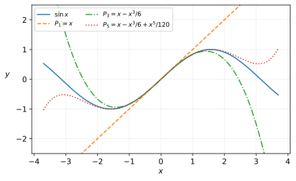
A tangent line matches a function’s value and first derivative at one input. A Taylor polynomial matches more derivatives:

P_n(x)=\sum_{k=0}^n\frac{f^{(k)}(a)}{k!}(x-a)^k.

The center is $a$ ; $a=0$ gives a Maclaurin polynomial. The polynomial is an exact algebraic object. Its use as $f(x)\approx P_n(x)$ is an approximation that needs an error discussion. The infinite Taylor series equals $f$ only where its remainders tend to zero.

C. A theorem that quantifies what is omitted#

If $f$ has continuous derivatives through order $n+1$ on an interval containing $a$ and $x$ , Taylor’s theorem gives

f(x)=P_n(x)+R_n(x),\qquad R_n(x)=\frac{f^{(n+1)}(\xi)}{(n+1)!}(x-a)^{n+1}

for some intermediate $\xi$ when $x\ne a$ . Therefore if $|f^{(n+1)}(t)|\le M$ throughout the intervening interval,

|R_n(x)|\le\frac{M|x-a|^{n+1}}{(n+1)!}.

The unknown $\xi$ is not a freely selected point and is not generally the endpoint. The notation $O((x-a)^m)$ , used later in the solutions, means a remainder whose magnitude is at most $C|x-a|^m$ for some fixed constant $C$ in a neighborhood of $a$ . It abbreviates a bound, not a claim that the remainder is zero. This is the Lagrange remainder form under convenient sufficient hypotheses. [O2Taylor]

Useful Maclaurin series are

e^x=\sum_{n=0}^{\infty}\frac{x^n}{n!},\quad \sin x=\sum_{n=0}^{\infty}\frac{(-1)^n x^{2n+1}}{(2n+1)!},\quad \cos x=\sum_{n=0}^{\infty}\frac{(-1)^n x^{2n}}{(2n)!},

valid for all real $x$ . The logarithmic series is $\ln(1+x)=\sum_{n=1}^{\infty}(-1)^{n-1}x^n/n$ for $-1<x\le1$ , with endpoint value justified separately. The geometric series has $|x|<1$ . Substituting into these identities requires checking their resulting domains.

D. Why the coefficients have factorial denominators#

At the center, derivatives of $(x-a)^k$ vanish until the $k$ th derivative, which equals $k!$ . Thus a coefficient $c_k$ contributes $k!c_k$ to the $k$ th derivative at $a$ . To match $f^{(k)}(a)$ , one must choose $c_k=f^{(k)}(a)/k!$ . The coefficients are forced by derivative matching, not guessed to fit a plotted curve.

The remainder theorem can be proved using repeated Rolle-type reasoning or repeated integration of the fundamental theorem. It isolates the first derivative order not already matched by the polynomial. For sine and cosine, derivatives stay bounded by one, while factorial denominators beat fixed powers; hence the remainders tend to zero. Smoothness alone is insufficient in general. The optional example $f(x)=e^{-1/x^2}$ for $x\ne0$ , $f(0)=0$ , has all derivatives zero at zero but is positive elsewhere. Its Taylor series is identically zero, so it does not represent the function away from the center.

E. A practical approximation procedure#

Choose a center with easy derivative values near the desired input. Build enough terms to meet the requested order, noting that a degree-three polynomial may have no cubic term. Choose an error method: Lagrange’s bound for a derivative-controlled interval, an alternating next-term bound when its hypotheses hold, or a geometric remainder for a geometric expansion. Keep exact expressions until the end and distinguish the certified error from the actual observed error. To evaluate a limit, enough leading terms plus a remainder estimate can justify which terms dominate.

F. Worked examples#

A logarithmic estimate. Using $x=0.2$ , the three-term polynomial gives $\ln(1.2)\approx0.2-0.2^2/2+0.2^3/3=137/750\approx0.182667$ . The alternating remainder magnitude is at most $0.2^4/4=0.0004$ , and the next term is negative, so this is an overestimate. The decimal itself is not an accuracy guarantee; the omitted-tail theorem is.

A shifted polynomial. For $f(x)=\sqrt x$ at $a=4$ , $f(4)=2$ , $f'(4)=1/4$ , and $f''(4)=-1/32$ . Hence $P_2(x)=2+(x-4)/4-(x-4)^2/64$ . The quadratic coefficient is $f''(4)/2!$ , not just $f''(4)$ .

Exact sine and its degree-one, degree-three, and degree-five Maclaurin polynomials. Their agreement is local; polynomial error must be evaluated on the input interval actually used. This plot illustrates behavior but does not prove a remainder bound.

Computing bridge: Local polynomial models and controlled extrapolation#

A Taylor polynomial is a local model whose domain of useful accuracy depends on the omitted terms. It can support finite-difference error estimates, local optimization, or a small-motion approximation, but it is not automatically reliable far from its center. In A05, truncation error competes with floating-point error; in T05, discretization error accumulates over time. The transferable habit is to state a region, an error measure, and a bound or convergence experiment before trusting a polynomial surrogate.

G. Independent practice#

F foundation C standard course work T transfer S optional stretch L runnable lab or project. Attempt the complete set before opening its solutions.

M30.01FSolution

Find the degree-four Maclaurin polynomial for $e^{2x}$ .

M30.02CSolution

Use $1-x^2/2$ to estimate $\cos(0.2)$ and give a bound using the first omitted nonzero term.

M30.03TSolution

Find the degree-three Taylor polynomial of $\ln x$ about $a=1$ . Bound its error at $x=1.1$ using Lagrange’s form.

M30.04CSolution

Use the sine series to evaluate $\lim_{x\to0}(\sin x-x+x^3/6)/x^5$ , explaining why the remainder disappears.

M30.05TSolution

Choose a sufficient degree $n$ to approximate $e^{0.5}$ by its degree- $n$ Maclaurin polynomial with error below $10^{-5}$ , using $e^t<2$ on $[0,0.5]$ .

M30.06TSolution

Find a series for $x^2e^{-x^2}$ and use its first three nonzero terms to approximate $\int_0^{1/2}x^2e^{-x^2}\dd x$ . Bound the error by an alternating term.

M30.07CSolution

Find the degree-two Taylor polynomial of $f(x)=1/x$ at $a=2$ , and use it to estimate $1/2.1$ .

M30.08SSolution

Explain why matching every derivative at a point need not imply two smooth functions agree near that point. For the flat function described above, justify $f'(0)=0$ directly and describe why its higher derivatives also vanish.

Optional small hints

For M30.03, $f^{(4)}(x)=-6/x^4$ . For M30.04, use a sine expansion through degree five with a higher-order remainder. For M30.06, integrate the series term by term on an interval strictly within its infinite radius.

H. Complete solutions: Module 30#

Compare the first step where your work differs. A corrected answer is not yet an independent success.

M30.01Show solution

Substitute into a known entire series

From $e^z=1+z+z^2/2!+z^3/3!+z^4/4!+\cdots$ , put $z=2x$ . The polynomial is

\boxed{1+2x+2x^2+\frac43x^3+\frac23x^4}.

The degree counts powers of $x$ , not how many terms were written. The exponential equals its infinite series, while this finite polynomial is an approximation away from zero.

Back to M30.01

M30.02Show solution

Use the first omitted nonzero term

The estimate is $1-0.2^2/2=\boxed{0.98}$ . The cosine series at this input alternates with decreasing magnitudes, so the error is at most $0.2^4/4!=\boxed{1/15000\approx0.00006667}$ . The next term is positive, so the true cosine lies between $0.98$ and $0.98006667$ . Treating the zero cubic coefficient as a zero error would be invalid.

Back to M30.02

M30.03Show solution

A derivative bound across the whole interval

At $1$ , the first three derivatives are $1,-1,2$ and the value is zero. Thus $P_3=(x-1)-(x-1)^2/2+(x-1)^3/3$ . On $[1,1.1]$ , $|f^{(4)}(x)|=6/x^4\le6$ . The remainder at $1.1$ is bounded by $6(0.1)^4/4!=\boxed{0.000025}$ . The polynomial value is $0.1-0.005+0.001/3\approx0.0953333$ . The bound, not the number of displayed decimals, specifies its guaranteed accuracy.

Back to M30.03

M30.04Show solution

Cancellation exposes the first surviving term

Taylor’s theorem gives $\sin x=x-x^3/6+x^5/120+O(x^7)$ near zero; the bound follows from bounded sine/cosine derivatives using the degree-six polynomial. Subtracting the displayed linear and cubic terms leaves $x^5/120+O(x^7)$ . Division by $x^5$ for $x\ne0$ gives $1/120+O(x^2)\to\boxed{1/120}$ . The remainder statement justifies dropping higher powers rather than treating an approximation as an exact equality.

Back to M30.04

M30.05Show solution

Solve a factorial error inequality

The bound is $2(0.5)^{n+1}/(n+1)!$ . At $n=5$ it is $2/(64\cdot720)\approx4.34\times10^{-5}$ , too large. At $n=6$ it is $2/(128\cdot5040)\approx3.10\times10^{-6}$ , below the target. Therefore $\boxed{n=6}$ is a sufficient degree using this bound. No claim is made that the actual degree-five error necessarily exceeds the target without calculating it.

Back to M30.05

M30.06Show solution

Substitute, multiply, integrate, then bound the new series

The representation is $x^2e^{-x^2}=\sum_{n=0}^{\infty}(-1)^n x^{2n+2}/n!$ , valid for all real $x$ . Integrating the first three terms gives

I\approx\left[x^3/3-x^5/5+x^7/14\right]_0^{1/2} =\frac1{24}-\frac1{160}+\frac1{1792}=\boxed{\frac{967}{26880}\approx0.0359747}.

The integrated series alternates with decreasing magnitudes. Its next term magnitude is $(1/2)^9/(6\cdot9)=\boxed{1/27648\approx0.00003617}$ . It is negative, so the estimate is above the true integral. The validity of termwise integration follows from convergence on this compact interval inside the infinite radius.

Back to M30.06

M30.07Show solution

A shifted geometric pattern provides a check

For $f=1/x$ , $f(2)=1/2$ , $f'(2)=-1/4$ , and $f''(2)=1/4$ . Thus $P_2(x)=1/2-(x-2)/4+(x-2)^2/8$ . At $2.1$ , this gives $\boxed{0.47625}$ . Independently, $1/x=(1/2)/[1+(x-2)/2]$ has a geometric expansion whose first three terms match this polynomial. The exact reciprocal is $10/21\approx0.4761905$ , so the observed error is about $0.0000595$ .

Back to M30.07

M30.08Show solution

Infinite smoothness is not analyticity

For the flat function, the difference quotient at zero is $e^{-1/h^2}/h$ . Its magnitude tends to zero because exponential decay in $1/h^2$ dominates the power $1/|h|$ ; hence $f'(0)=0$ . Away from zero, repeated derivatives have the form a polynomial in $1/x$ times $e^{-1/x^2}$ . Every such expression tends to zero as $x\to0$ , and its divided-by- $x$ versions do too, allowing an induction that all derivatives at zero exist and vanish. Thus its Taylor coefficients agree with the zero function’s coefficients, but $f(x)>0$ for $x\ne0$ . Derivative matching alone is not equality to the Taylor series; the remainder must tend to zero at the input in question.

Back to M30.08

I. Retention and readiness#

Revisit M13.01, M23.03, and M29.08. Explain whether a displayed equality is a finite polynomial identity, a convergent infinite-series identity, or an approximation with a remainder. Advance when you can justify how many terms are enough for a requested accuracy.